BBRKC GMACS to RTMB Porting Notes

Purpose

This document tracks the staged conversion of the BBRKC GMACS ADMB model to an RTMB implementation. The current goal is not to translate all of gmacs.tpl at once. The goal is to create a reproducible sequence of parity checks where each deterministic model block is ported and compared with existing ADMB output before the corresponding likelihood components are activated.

The BBRKC case is read from examples/BBRKC and currently uses:

• gmacs.dat for file routing and run controls.
• bbrkc_21_1.dat for dimensions, catch, survey, composition, growth, and environmental data.
• bbrkc_21_1.ctl for phases, selectivity structure, mortality controls, and likelihood weights.
• gmacs.pin for the fitted full parameter state.
• gmacs.rep and Gmacsall.out as ADMB parity references.

Current RTMB Files

The current scaffold lives at the repository root.

File	Role
R/read_gmacs_bbrkc.R	Reads BBRKC GMACS inputs, fitted .pin values, ADMB likelihood blocks, selectivity reports, mortality reports, growth reports, and numbers-at-size reports.
R/gmacs_rtmb_nll.R	Builds RTMB data and parameter lists, maps full .pin values to active parameters, and contains deterministic model blocks.
run_bbrkc.R	Runs parser validation, constructs the mapped RTMB object, and prints deterministic parity diagnostics.
optimize_bbrkc.R	Runs a short nlminb() optimization smoke test from the mapped 366-parameter RTMB object.

Parameter Mapping

The full BBRKC .pin file contains 560 numeric entries. ADMB reports 366 active estimated parameters. The function make_bbrkc_rtmb_map() builds an RTMB map from the BBRKC control phases and maps inactive entries to NA.

Special cases:

• log_fdev and log_fdov activity follows the corresponding fleet-level log_fbar and log_foff phases.
• log_vn uses the GMACS composition aggregator, reducing 13 input composition controls to 8 effective sample-size entries.
• logit_rec_prop_est is treated like an ADMB dev vector, so one element is mapped off to reproduce 45 active entries from 46 values.
• BBRKC uses FREEPARSSCALED initial numbers. The first scaled logN0 entry is fixed at zero and theta[13:91] supplies the remaining 79 sex/shell/size offsets.

Expected check:

source("R/read_gmacs_bbrkc.R")
source("R/gmacs_rtmb_nll.R")

inputs <- read_bbrkc_inputs("examples/BBRKC")
map <- make_bbrkc_rtmb_map(inputs)
count_active_map_parameters(map)

Expected result: 366.

Deterministic Status

The current RTMB scaffold ports BBRKC selectivity, fishing mortality, natural mortality, total mortality/survival setup, growth, recruitment, initial numbers, the annual/seasonal population update, catch predictions, and catch-at-size predictions. Catch, robust size-composition, and recruitment likelihoods are now active in the RTMB objective and checked against the ADMB nloglike reference. Survey/index predictions and likelihoods are now active and matched against the ADMB #Index_fit_summary and raw nloglike reference.

Block	RTMB function	ADMB reference	Status
Parameter map	make_bbrkc_rtmb_map()	ADMB active parameter count	560 .pin entries mapped to 366 active parameters
Capture selectivity	calc_bbrkc_capture_selectivity()	gmacs.rep, slx_capture	Matches report rounding
Retention and discard selectivity	calc_bbrkc_retention_selectivity()	gmacs.rep, slx_retaind, slx_discard	Matches report rounding
Fishing mortality	calc_bbrkc_fishing_mortality()	Gmacsall.out, fully selected F and continuous F-at-size	Matches ADMB numerical output
Natural mortality	calc_bbrkc_natural_mortality()	Gmacsall.out, natural mortality by class	Matches ADMB numerical output
Total mortality	calc_bbrkc_total_mortality()	Gmacsall.out, continuous and discrete total mortality by class	Matches ADMB numerical output
Molt probability	calc_bbrkc_molting_probability()	Gmacsall.out, molt probability	Matches ADMB numerical output
Growth transition	calc_bbrkc_growth_transition()	Gmacsall.out, growth transition matrix	Matches ADMB numerical output and uses RTMB::pgamma() so active growth parameters affect the tape
Recruitment	calc_bbrkc_recruits()	Gmacsall.out, overall summary	Matches ADMB numerical output to printed precision
Initial numbers	calc_bbrkc_initial_numbers()	Gmacsall.out, N(...) at first output season	FREEPARSSCALED normalized logN offsets ported
Population update	calc_bbrkc_population_numbers()	Gmacsall.out, N(total), sex, and shell blocks	Matches ADMB numerical output to printed precision
Catch observations	calc_bbrkc_predicted_catch()	Gmacsall.out, Catch_fit_summary	Matches ADMB numerical output to printed precision; AD-safe flat vector is taped and reported
Catch-at-size	calc_bbrkc_predicted_size_compositions()	Gmacsall.out, Size_fit_summary	Matches ADMB numerical output to printed precision; AD-safe flat vector is taped and reported
Catch likelihood	catch_likelihood() inside gmacs_rtmb_nll_factory()	Gmacsall.out, nloglike row 1	Matches ADMB raw likelihood components
Survey index	calc_bbrkc_predicted_survey()	Gmacsall.out, #Index_fit_summary	Matches ADMB predicted index output to printed precision
Survey likelihood	index_likelihood() inside gmacs_rtmb_nll_factory()	Gmacsall.out, nloglike row 2	Matches ADMB raw likelihood components
Length likelihood	length_likelihood() inside gmacs_rtmb_nll_factory()	Gmacsall.out, nloglike row 3	Robust multinomial likelihood matches ADMB raw components
Recruitment likelihood	recruitment_likelihood() inside gmacs_rtmb_nll_factory()	Gmacsall.out, nloglike row 4	Uses ADMB-style res_recruit; matches ADMB raw components
Penalties	calc_bbrkc_penalties()	Gmacsall.out, nlogPenalty	Raw penalty vector matches ADMB; weighted vector enters the RTMB objective
Priors	calc_bbrkc_prior_density()	Gmacsall.out, priorDensity	Prior-density vector matches ADMB and enters the RTMB objective

Selectivity Details

Capture selectivity:

• All BBRKC capture components are logistic.
• Logistic curves are normalized to the terminal size class because the control file sets slx_max_at_1 = 1.
• NMFS trawl selectivity is embedded within BSFRF selectivity, matching slx_incl = 6.

Retention selectivity:

• Pot fishery male retention is logistic.
• The Pot male retention curve changes parameter block in 2005.
• Pot female and all non-Pot retention components are effectively zero retention for BBRKC.
• Discard selectivity is computed as log(1 - retained + 1e-08), matching the ADMB template.
• The 1975 Pot male high-grading adjustment from Asymret is applied.

Current parity command:

Rscript run_bbrkc.R

Current expected selectivity differences are on the order of GMACS report rounding:

Component	Maximum absolute difference
Capture selectivity	about 5e-05
Retained selectivity	about 4e-05
Discard selectivity	about 4e-05

Mortality Details

Fishing mortality:

• log_fbar supplies the fleet-level mean fishing mortality.
• log_fdev supplies male annual/seasonal deviations for each fleet.
• Female F uses the fleet-level log_foff offset and the active log_fdov deviations where female catches occur.
• Vulnerability is computed from capture selectivity, retention selectivity, and discard mortality.
• Both fully selected F and continuous F-at-size are compared with Gmacsall.out.

Natural mortality:

• BBRKC uses GMACS natural mortality type 6.
• Male base M is theta[1].
• Female base M is relative to male M through theta[2].
• The control file defines two natural-mortality nodes per sex, with the first deviation active over 1980-1984.
• Mdev_spec = -1 shares the first male M-deviation parameter with the female block, matching the ADMB template.
• No BBRKC size-specific M multiplier is active.

Total mortality:

• Continuous total mortality is Z = m_prop * M + F.
• Discrete total mortality is Z2 = m_prop * M + F2.
• The survival diagonal S is computed from Z for the BBRKC season type.

Growth Details

Growth parameter unpacking:

• BBRKC uses growth transition option 3, where growth increments are gamma distributed.
• The growth increment model is empirical by size class.
• Male growth has one transition block.
• Female growth has three transition blocks, with changes in 1983 and 1994.
• Gscale is handled with the BBRKC relative-beta setting, so female periods 2 and 3 inherit the period-1 scale when their fitted relative values are zero.

Molt probability:

• BBRKC uses logistic molt probability.
• Both sexes define two molt-probability blocks, with a change in 1980.
• Female fitted values make molt probability effectively one for all modeled sizes and years.

Growth transition:

• The transition matrix is computed from active growth parameters using the GMACS gamma-increment formula.
• GMACS prints trans(growth_transition), so the ADMB parser explicitly treats printed rows as destination size classes and printed columns as source size classes.
• Gamma CDF calls use RTMB::pgamma() through the local ad_pgamma() wrapper, avoiding the previous numeric precompute from gmacs.pin.

Recruitment and Population Details

Recruitment:

• Annual recruitment is split by sex with logit_rec_prop_est, matching the ADMB dev-vector indexing.
• The first-year initial recruits use logRini for FREEPARSSCALED initial numbers.
• Recruitment size distribution is computed from the GMACS gamma recruitment formula and truncated at the sex-specific maximum recruitment size.
• Recruitment size probabilities also use RTMB::pgamma() through ad_pgamma(), so the distribution responds to active theta recruitment size parameters on the tape.

Initial numbers:

• The group order follows the ADMB loops over sex, maturity, and shell.
• For BBRKC this produces four groups: male new shell, male old shell, female new shell, and female old shell.
• The first logN0 offset is fixed at zero; the remaining 79 offsets are read from theta[13:91].
• Initial numbers are normalized as exp(logRini + logN0) / sum(exp(logN0)).

Population update:

• BBRKC uses the GMACS Case-D branch: two shell conditions, one maturity state, and no terminal molt.
• Survival is applied before growth and recruitment.
• In the growth season, molting crabs transition through the sex- and period-specific growth matrix; new-shell nonmolters become old-shell crabs.
• In the recruitment season, recruits enter the new-shell group by sex and recruitment size distribution.
• Output comparisons use season_N from the data file and compare total, sex-specific, and shell-specific numbers-at-size.

Catch Prediction Details

Mean weight:

• BBRKC uses length-weight input type 2: fixed mean weight-at-size vectors by sex and maturity.
• The RTMB parser reads mean weight, maturity, and legal vectors from the control file because catch observations are in mass units.

Catch observations:

• calc_bbrkc_predicted_catch() ports the Baranov prediction in calc_predicted_catch().
• Retained catch uses capture selectivity times retention.
• Discarded catch uses capture selectivity times one minus retention.
• Total catch uses capture selectivity alone.
• Sex-specific and combined-sex catch rows are both handled.
• Catch rows with zero observed catch and positive effort use the GMACS catchability calculation for obs_catch_effort.

Catch-at-size:

• calc_bbrkc_predicted_size_compositions() ports the catch-like branch of calc_predicted_composition().
• The function predicts each of the 13 input composition series, then applies the GMACS composition appender to produce the 8 modified series used in the likelihood and report.
• Series with lf_catch_in == 2 are survey-like composition predictions and use numbers at size without the catch mortality multiplier.
• The 2021 season-1 survey-like size-composition rows use the propagated nyr + 1 population state and the terminal modeled-year selectivity.

Taping status:

• Catch and catch-at-size prediction helpers now use AD-compatible vector construction.
• MakeADFun() tapes these predictions and reports model$pre_catch, model$res_catch, model$log_q_catch, and model$pre_size_comps.
• The composition report is flattened and accompanied by model$size_comp_rows and model$size_comp_cols, which reconstruct the 8 modified composition series.

Next Porting Steps

1. Prediction Blocks

Port or refine the remaining deterministic and objective blocks in this order:

1. Survey-like size-composition branch review for lf_catch_in == 2, using the now-active survey prediction logic as a guide.
2. Optional growth likelihood scaffolding if active growth observations are introduced.
3. Broader validation against additional GMACS model configurations.

These should continue to be checked in small pieces against Gmacsall.out and gmacs.rep before likelihood components are activated.

2. Predictions and Likelihoods

The active likelihood blocks are:

• catch likelihood
• survey index likelihood
• robust length-composition likelihood
• recruitment likelihood

Remaining likelihood work:

• survey-like size-composition likelihood checks after survey composition predictions are reconciled
• growth likelihood only if active growth observations are introduced

run_bbrkc.R now performs this audit directly after taping the objective. Each deterministic prediction change should be followed by a run that compares the active nloglike components, raw nlogPenalty, and priorDensity vectors against the ADMB blocks read from Gmacsall.out.

Optimization Smoke Test

The short optimizer smoke test uses the same BBRKC parser, mapped parameter list, RTMB objective, and 366-parameter map. It is intentionally capped at a small number of iterations so it checks that the taped objective and gradient are usable without treating the result as a production fit.

Rscript optimize_bbrkc.R

Current smoke-test output:

active parameter length: 366
initial objective: -25377.33
finite gradient: TRUE
max abs gradient: 28.4894
optimizer convergence: 1
optimizer message: iteration limit reached without convergence (10)
final objective: -25393.89
objective change: -16.55864

Run Log

The current successful run reports:

mapped active parameters: 366
RTMB object taped
active parameter length: 366
initial objective: -25377.33
likelihood components:
  catch RTMB=-271.2013 ADMB=-271.2013 diff=1.977e-07
  index RTMB=-37.85266 ADMB=-37.85266 diff=5.767e-07
  length RTMB=-25524.42 ADMB=-25524.42 diff=-3.529e-07
  recruitment RTMB=145.2397 ADMB=145.2397 diff=-6.589e-08
  growth RTMB=0 ADMB=0 diff=0
raw penalty max abs diff: 1.023e-06
raw penalty sum: 4995.897
weighted penalty sum: 43.9388
prior density max abs diff: 1.548e-07
prior density sum: 266.9703
capture selectivity max abs diff: 4.972e-05
retained selectivity max abs diff: 4.164e-05
discard selectivity max abs diff: 4.163e-05
fully selected F max abs diff: 3.347e-08
F at size max abs diff: 2.037e-08
natural mortality max abs diff: 4.575e-09
continuous total mortality max abs diff: 2.037e-08
discrete total mortality max abs diff: 4.235e-08
molt probability max abs diff: 6.996e-09
growth transition max abs diff: 8.162e-09
recruits max abs diff: 1.947
N(total) max abs diff: 1.784
N(males) max abs diff: 0.438
N(females) max abs diff: 1.742
N(males_new) max abs diff: 0.438
N(females_new) max abs diff: 1.742
N(males_old) max abs diff: 0.1004
N(females_old) max abs diff: 2.993e-37
catch predicted max abs diff: 7.484e-05
catch residual max abs diff: 1.145e-08
index predicted max abs diff: 0.0006836
index q max abs diff: 1.483e-05
size composition predicted max abs diff: 4.999e-05

The current RTMB objective includes catch, survey index, length-composition, and recruitment likelihoods plus the weighted ADMB penalty contribution. Raw likelihood components match the ADMB nloglike block, and raw penalty components match the ADMB nlogPenalty block to printed precision. The priorDensity vector is active and matches ADMB to numerical precision. The abundance differences above are on the scale of individual crabs while the reported arrays contain millions, so they are consistent with ADMB text-output precision.

Appendix: Model Equations

This appendix records the equation set represented by the current RTMB scaffold and the remaining GMACS equations that still need to be activated. The conversion is not complete, but the BBRKC population dynamics, growth transition matrices, recruitment size distributions, catch predictions, catch-at-size predictions, catch likelihood, robust length-composition likelihood, survey index likelihood, and recruitment likelihood are ported and taped; weighted penalties and prior densities are active.

A. Notation

Indices:

• \(i\) indexes model years.
• \(j\) indexes seasons.
• \(h\) indexes sex.
• \(m\) indexes maturity state.
• \(o\) indexes shell state.
• \(g = (h,m,o)\) indexes the combined GMACS population group.
• \(\ell\) indexes size classes.
• \(k\) indexes fisheries or survey fleets.
• \(r\) indexes rows in the observation tables.
• \(a\) indexes modified size-composition series after GMACS aggregation.

Main state and prediction quantities:

• \(N_{g,i,j,\ell}\) is abundance at size at the start of year \(i\) and season \(j\).
• \(S_{k,h,i,\ell}\) is capture selectivity.
• \(R_{k,h,i,\ell}\) is retention probability.
• \(V_{k,h,i,\ell}\) is the fully selected fishing mortality multiplier at size.
• \(F_{h,i,j,\ell}\) is fishing mortality at size after summing over active fleets.
• \(M_{h,m,i,\ell}\) is natural mortality at size.
• \(Z_{h,m,i,j,\ell}\) is total mortality for continuous seasons.
• \(G_{h,i,\ell,\ell'}\) is the growth transition matrix.
• \(P^{\mathrm{molt}}_{h,i,\ell}\) is molt probability.
• \(\widehat{C}_r\) is predicted catch for observation row \(r\).
• \(\widehat{p}_{a,\ell}\) is predicted size composition for modified composition series \(a\).

BBRKC uses the four group states male-new, male-old, female-new, and female-old. Immature crab are not active in this model configuration, but the RTMB arrays preserve the GMACS group structure.

B. Population Dynamics

Leading Parameters

The male base natural mortality and female multiplier are represented by leading parameters:

\[ M^0_{\mathrm{male}} = \theta_1, \qquad M^0_{\mathrm{female}} = \theta_1 \exp(\theta_2). \]

Mean recruitment is parameterized on the log scale:

\[ \bar{R} = \exp(\theta_5). \]

R implementation: leading parameter unpacking

initialize_bbrkc_model_parameters <- function(par, data, predictions = TRUE) {
  theta <- par$theta
  m0 <- c(theta[1], theta[1] * exp(theta[2]))
  model <- list(
    M0 = m0,
    logR0 = theta[3],
    logRini = theta[4],
    logRbar = theta[5],
    logSigmaR = theta[10],
    rho = theta[12]
  )
  ...
}

Initial Abundance

GMACS stores the initial numbers-at-size as scaled free parameters. The RTMB port follows the ADMB convention by setting the first log-scale element to zero and reading the remaining elements from the active theta block:

\[ \log \widetilde{N}_{g,\ell} = \begin{cases} 0, & (g,\ell) = (1,1),\\ \theta_q, & \text{otherwise}. \end{cases} \]

Initial abundance is normalized and scaled by initial recruitment:

\[ N_{g,i_0,1,\ell} = \exp(\log R_{\mathrm{init}}) \frac{\exp(\log \widetilde{N}_{g,\ell})} {\sum_{g'}\sum_{\ell'} \exp(\log \widetilde{N}_{g',\ell'})}. \]

Recruitment

Annual recruitment deviations are additive on the log scale. Sex allocation is controlled by a logit-scale recruitment proportion:

\[ p_i = \operatorname{logit}^{-1}(\eta_i), \]

\[ R_{\mathrm{male},i} = 2 \exp(\log \bar{R} + d_i) p_i, \qquad R_{\mathrm{female},i} = 2 \exp(\log \bar{R} + d_i) (1 - p_i). \]

Recruitment enters the new-shell group according to the recruitment size distribution \(\rho_{h,\ell}\):

\[ N_{\mathrm{new},h,i,1,\ell} \leftarrow N_{\mathrm{new},h,i,1,\ell} + R_{h,i}\rho_{h,\ell}. \]

R implementation: recruitment and sex split

calc_bbrkc_recruits <- function(par, data, model) {
  rec_rows <- years >= controls$rdv_syr & years <= controls$rdv_eyr
  rec_dev[rec_rows] <- par$rec_dev_est[seq_len(sum(rec_rows))]
  logit_rec_prop[rec_rows] <- par$logit_rec_prop_est[seq_len(sum(rec_rows))]

  for (iy in seq_len(n_years)) {
    total_recruitment <- exp(model$logRbar) * nsex
    total_recruitment <- total_recruitment * exp(rec_dev[iy])
    male_prop <- 1 / (1 + exp(-logit_rec_prop[iy]))
    recruits[1, iy] <- total_recruitment * male_prop
    recruits[2, iy] <- total_recruitment * (1 - male_prop)
  }
}

Natural Mortality

For sex \(h\) and maturity state \(m\), natural mortality is

\[ M_{h,m,i,\ell} = M^0_h \exp(\delta_{h,b(i)}) Q_{h,m,\ell}, \]

where \(\delta_{h,b(i)}\) is the block-specific natural-mortality deviation and \(Q_{h,m,\ell}\) is an optional size-specific multiplier. In the current BBRKC input, the active size-specific multiplier is effectively one:

\[ Q_{h,m,\ell} = 1. \]

Selectivity, Retention, and Fishing Mortality

The port currently supports the logistic GMACS selectivity form used by the BBRKC fleets:

\[ s_{k,h,i,\ell} = \frac{ \left[1 + \exp\left\{-(L_\ell - x_{50,k,h,i})/\gamma_{k,h,i}\right\}\right]^{-1} } {\max_{\ell'} \left[1 + \exp\left\{-(L_{\ell'} - x_{50,k,h,i})/\gamma_{k,h,i}\right\}\right]^{-1}}, \]

where \(L_\ell\) is the size-bin midpoint, \(x_{50}\) is the size at 50 percent selection, and \(\gamma\) controls the slope. Retention uses the same logistic form with retention-specific parameters:

\[ r_{k,h,i,\ell} = \left[1 + \exp\left\{-(L_\ell - x^{R}_{50,k,h,i})/\gamma^R_{k,h,i}\right\}\right]^{-1}. \]

The fleet-specific availability multiplier combines capture selectivity, retention, and the high-grading or discard mortality term \(\xi_k\):

\[ V_{k,h,i,\ell} = s_{k,h,i,\ell} \,\left[ r_{k,h,i,\ell} + (1-r_{k,h,i,\ell})\xi_k \right]. \]

Fully selected fleet mortality is

\[ f_{k,h,i,j} = \exp(\log f_{k,h,i,j}), \]

and total fishing mortality at size is summed over active fleets:

\[ F_{h,i,j,\ell} = \sum_k f_{k,h,i,j} V_{k,h,i,\ell}. \]

R implementation: selectivity, retention, and fishing mortality

calc_bbrkc_fishing_mortality <- function(par, data, model) {
  for (fleet in seq_len(nfleet)) {
    for (sex in seq_len(nsex)) {
      ...
      sel <- exp(model$log_slx_capture[fleet, sex, iy, ]) + 1e-10
      ret <- exp(model$log_slx_retaind[fleet, sex, iy, ]) * slx_nret[sex, fleet]
      vul <- sel * (ret + (1 - ret) * xi)
      F[sex, iy, season, ] <- F[sex, iy, season, ] +
        ft[fleet, sex, iy, season] * vul
      F2[sex, iy, season, ] <- F2[sex, iy, season, ] +
        ft[fleet, sex, iy, season] * sel
    }
  }
}

Total Mortality and Survival

Continuous-season total mortality is

\[ Z_{h,m,i,j,\ell} = \tau^M_j M_{h,m,i,\ell} + F_{h,i,j,\ell}, \]

where \(\tau^M_j\) is the proportion of annual natural mortality applied in season \(j\). Survival through the season is

\[ \phi_{h,m,i,j,\ell} = \exp(-Z_{h,m,i,j,\ell}). \]

For discrete-season accounting, GMACS also stores the equivalent annualized total mortality used for reporting:

\[ Z^{D}_{h,m,i,j,\ell} = \frac{-\log\left[ 1 - \left[ 1 - \exp\left\{ -(\tau^M_j M_{h,m,i,\ell} + F_{h,i,j,\ell}) \right\} \right] \right]} \tau_j, \]

where \(\tau_j\) is the modeled season length.

Molting and Growth

The molt probability is represented as a declining logistic curve:

\[ P^{\mathrm{molt}}_{h,i,\ell} = 1 - \left[ 1 + \exp\left\{-\frac{L_\ell-\mu^{\mathrm{molt}}_{h,i}} {\sigma^{\mathrm{molt}}_{h,i}}\right\} \right]^{-1}. \]

Growth is represented by a transition matrix \(G_{h,i,\ell,\ell'}\):

\[ G_{h,i,\ell,\ell'} = \Pr(L_{\ell'} \mid L_\ell,\ h,\ i), \qquad \sum_{\ell'} G_{h,i,\ell,\ell'} = 1. \]

The current RTMB port computes the same transition matrix as ADMB to text-output precision, using the BBRKC molt-increment controls and the same terminal-bin normalization.

R implementation: molt probability and growth transition

calc_bbrkc_molting_probability <- function(growth, data) {
  for (sex in seq_len(nsex)) {
    location <- growth$molt_mu[sex]
    scale <- growth$molt_mu[sex] * growth$molt_cv[sex]
    out[sex, ] <- 1 - plogis_gmacs(data$mid_points, location, scale)
  }
  out
}

calc_bbrkc_growth_transition <- function(growth, data) {
  for (sex in seq_len(nsex)) {
    for (from in seq_len(nclass)) {
      cdf <- ad_pgamma(data$size_breaks - data$mid_points[from],
        shape = shape[from], scale = scale
      )
      probs <- diff(cdf)
      out[sex, from, ] <- probs / sum(probs)
    }
  }
  out
}

Season and Year Propagation

Let post-mortality abundance be

\[ \widetilde{N}_{g,i,j,\ell} = N_{g,i,j,\ell}\phi_{h,m,i,j,\ell}. \]

For new-shell crab, the nonmolting component moves to old shell and the molting component remains new shell after growth:

\[ N^{\mathrm{old}}_{h,i,j+1,\ell} \leftarrow N^{\mathrm{old}}_{h,i,j+1,\ell} + \widetilde{N}^{\mathrm{new}}_{h,i,j,\ell} \left(1-P^{\mathrm{molt}}_{h,i,\ell}\right), \]

\[ N^{\mathrm{new}}_{h,i,j+1,\ell'} \leftarrow N^{\mathrm{new}}_{h,i,j+1,\ell'} + \sum_\ell \widetilde{N}^{\mathrm{new}}_{h,i,j,\ell} P^{\mathrm{molt}}_{h,i,\ell} G_{h,i,\ell,\ell'}. \]

For old-shell crab, the nonmolting component remains old shell and the molting component returns to new shell after growth:

\[ N^{\mathrm{old}}_{h,i,j+1,\ell} \leftarrow N^{\mathrm{old}}_{h,i,j+1,\ell} + \widetilde{N}^{\mathrm{old}}_{h,i,j,\ell} \left(1-P^{\mathrm{molt}}_{h,i,\ell}\right), \]

\[ N^{\mathrm{new}}_{h,i,j+1,\ell'} \leftarrow N^{\mathrm{new}}_{h,i,j+1,\ell'} + \sum_\ell \widetilde{N}^{\mathrm{old}}_{h,i,j,\ell} P^{\mathrm{molt}}_{h,i,\ell} G_{h,i,\ell,\ell'}. \]

At the terminal season, the propagated state becomes the first season of the next modeled year.

R implementation: population update

calc_bbrkc_population_numbers <- function(par, data, model) {
  for (iy in seq_len(n_years)) {
    for (season in seq_len(nseason)) {
      for (group in seq_len(n_groups)) {
        survived <- N[group, iy, season, ] * model$S[sex, maturity, iy, season, ]
        molted <- survived * model$molt_probability[sex, ]
        not_molted <- survived * (1 - model$molt_probability[sex, ])
        grown <- as.vector(molted %*% model$growth_transition[sex, , ])
        ...
      }
    }
  }
}

C. Observation and Prediction Equations

Catch Predictions

For catch observation row \(r\), let \(k(r)\) be the fleet, \(i(r)\) the year, \(j(r)\) the season, \(H_r\) the included sexes, and \(T_r\) the catch type. The catch-type availability is

\[ A^{T_r}_{k,h,i,\ell} = \begin{cases} s_{k,h,i,\ell}, & T_r = \mathrm{capture},\\ s_{k,h,i,\ell} r_{k,h,i,\ell}, & T_r = \mathrm{retained},\\ s_{k,h,i,\ell} (1-r_{k,h,i,\ell}), & T_r = \mathrm{discard}. \end{cases} \]

Predicted catch uses the Baranov catch equation:

\[ \widehat{C}_r = \sum_{h \in H_r}\sum_m\sum_o\sum_\ell W^{u_r}_{h,m,\ell} N_{h,m,o,i(r),j(r),\ell} f_{k(r),h,i(r),j(r)} A^{T_r}_{k(r),h,i(r),\ell} \frac{1-\exp[-Z_{h,m,i(r),j(r),\ell}]} {Z_{h,m,i(r),j(r),\ell}}, \]

where \(u_r\) determines whether the observation is in numbers or biomass:

\[ W^{u_r}_{h,m,\ell} = \begin{cases} 1, & u_r = \mathrm{numbers},\\ w_{h,m,\ell}, & u_r = \mathrm{biomass}. \end{cases} \]

The catch residual currently reported by RTMB is

\[ e^{C}_r = \log(C^{\mathrm{obs}}_r) - \log(\widehat{C}_r). \]

When GMACS treats catch as effort with analytic catchability, the same predicted catch vector is used to estimate

\[ \log \widehat{q}_r = \log(C^{\mathrm{obs}}_r) - \log(\widehat{C}_r). \]

R implementation: catch prediction

calc_bbrkc_predicted_catch <- function(data, model) {
  for (series in seq_along(data$catch$frames)) {
    for (row in seq_len(nrow(frame))) {
      ...
      nal <- calc_bbrkc_catch_weighted_numbers(
        model, data, sex, maturity, group, year_index, season, units
      )
      mult <- calc_bbrkc_catch_mortality_multiplier(
        model, data, sex, maturity, year_index, season
      )
      pre <- pre + sum(nal * model$ft[fleet, sex, year_index, season] * sel * mult)
      residual <- log(cobs) - log(pre)
    }
  }
}

Size-Composition Predictions

For catch-like size-composition rows, the unnormalized predicted count at size uses the same catch mortality multiplier as the catch equation:

\[ D_{r,\ell} = \sum_{h \in H_r}\sum_m\sum_o N_{h,m,o,i(r),j(r),\ell} f_{k(r),h,i(r),j(r)} A^{T_r}_{k(r),h,i(r),\ell} \frac{1-\exp[-Z_{h,m,i(r),j(r),\ell}]} {Z_{h,m,i(r),j(r),\ell}}. \]

For survey-like size-composition rows, the prediction is based on selected numbers at size:

\[ D_{r,\ell} = \sum_{h \in H_r}\sum_m\sum_o N_{h,m,o,i(r),j(r),\ell} A^{T_r}_{k(r),h,i(r),\ell}. \]

After optional tail compression, rows assigned to the same modified composition series \(a\) are accumulated and normalized:

\[ \widehat{p}_{a,\ell} = \frac{\sum_{r \in a} D_{r,\ell}} {\sum_{\ell'}\sum_{r \in a} D_{r,\ell'}}. \]

The current RTMB report stores this as a flat vector model$pre_size_comps, with dimensions carried by model$size_comp_rows and model$size_comp_cols.

R implementation: size-composition prediction and aggregation

calc_bbrkc_predicted_size_compositions <- function(data, model) {
  for (series in seq_len(n_input)) {
    ...
    if (controls$lf_catch_in[series] == 1L) {
      mult <- calc_bbrkc_catch_mortality_multiplier(...)
    } else {
      mult <- rep(1, data$dimensions[["nclass"]])
    }
    dntmp <- dntmp + model$N[group, year_index, season, ] * sel * mult
  }

  for (modified in seq_len(n_modified)) {
    input_series <- which(controls$comp_aggregator == modified)
    row_pred <- do.call(c, row_values)
    pred_rows[[row]] <- row_pred / sum(row_pred)
  }
}

Survey Index Predictions

Survey abundance and biomass predictions are active in RTMB. For survey row \(r\), the vulnerable selected abundance or biomass before catchability scaling is

\[ V_r = \sum_{h \in H_r}\sum_m\sum_o\sum_\ell W^{u_r}_{h,m,\ell} N_{h,m,o,i(r),j(r),\ell} B_{k(r),h,i(r),\ell}, \]

where \(B_{k,h,i,\ell}\) is survey selectivity, optionally including retention or other survey-specific availability modifiers depending on the GMACS survey type. If the survey occurs after part of the season has elapsed, the selected numbers are discounted by \(\exp(-t_r Z_{h,m,i,j,\ell})\) before summation.

Predicted index is

\[ \widehat{I}_r = q_{s(r)} V_r, \]

where \(s(r)\) is the survey series. For analytic catchability,

\[ \log \widehat{q}_{k} = \frac{ \sum_{r \in k} \omega_r \left[\log(I^{\mathrm{obs}}_r) - \log(\widehat{I}_r/q_k)\right] }{ \sum_{r \in k} \omega_r }. \]

The BBRKC run currently estimates or fixes survey q directly from the .pin state rather than using analytic q. The reported RTMB model$pre_cpue vector is checked against #Index_fit_summary in Gmacsall.out.

R implementation: survey prediction

calc_bbrkc_predicted_survey <- function(par, data, model) {
  for (row in seq_len(nrow(survey))) {
    ...
    survey_availability <- if (data$survey$index_type[series] == 2L) {
      sel * ret
    } else {
      sel
    }
    nal <- calc_bbrkc_survey_weighted_numbers(
      model, data, sex, maturity, group, year_index, season, units
    )
    row_v <- row_v + sum(nal * survey_availability * exp(-z_at_time))
  }

  pred <- survey_q_vec[series] * vulnerable_vec[row]
  pre_cpue[[row]] <- pred
  res_cpue[[row]] <- log(survey$obs[row]) - log(pred)
}

D. Model Fitting and Likelihoods

The current RTMB objective includes the likelihood components whose prediction vectors have been ported and validated:

\[ \mathcal{L} = \mathcal{L}_{\mathrm{catch}} + \mathcal{L}_{\mathrm{comp}} + \mathcal{L}_{\mathrm{survey}} + \mathcal{L}_{\mathrm{recruit}} + \mathcal{P}_{\mathrm{weighted}} + \mathcal{D}_{\mathrm{prior}} + 0_{\mathrm{growth}} \]

Weighted penalties and prior densities are active in the objective. Growth likelihood is zero because the current BBRKC data file has no active growth observations.

R implementation: objective assembly

nloglike <- c(
  catch = sum(catch_nloglike * data$likelihood_emphasis$catch),
  index = sum(index_nloglike * data$likelihood_emphasis$cpue_emphasis),
  length = sum(length_nloglike * data$observed_size_compositions$emphasis),
  recruitment = sum(recruitment_nloglike),
  growth = growth_nloglike
)

nll + sum(nloglike) + sum(weighted_nlog_penalty) + sum(prior_density)

Catch Likelihood

For lognormal catch observations,

\[ \sigma^C_r = \sqrt{\log(1 + \mathrm{cv}_{r}^{2})}, \qquad e^C_r = \log(C^{\mathrm{obs}}_r) - \log(\widehat{C}_r), \]

and the contribution is

\[ \mathcal{L}_{\mathrm{catch}} = \sum_r \lambda^C_r \left[ \frac{1}{2}\left(\frac{e^C_r}{\sigma^C_r}\right)^2 + \log(\sigma^C_r\sqrt{2\pi}) \right]. \]

Rows configured as effort observations use the same residual form after applying the analytic or estimated catchability parameter.

R implementation: catch likelihood

admb_dnorm_nll <- function(x, sd, mean = 0) {
  sum(0.5 * log(2 * pi) + log(sd) + 0.5 * ((x - mean) / sd)^2)
}

catch_likelihood <- function() {
  out <- vector("list", length(data$catch$frames))
  start <- 1L
  for (series in seq_along(data$catch$frames)) {
    frame <- data$catch$frames[[series]]
    rows <- nrow(frame)
    idx <- start:(start + rows - 1L)
    catch_sd <- sqrt(log(1 + frame$cv^2))
    out[[series]] <- admb_dnorm_nll(model$res_catch[idx], catch_sd)
    start <- start + rows
  }
  do.call(c, out)
}

Survey Likelihood

For lognormal survey index observations with optional additive process error,

\[ \sigma^I_r = \sqrt{\log\left(1 + \mathrm{cv}_{r}^{2}\right) + \sigma^2_{\mathrm{add},k(r)}}, \]

\[ e^I_r = \log(I^{\mathrm{obs}}_r) - \log(\widehat{I}_r), \]

\[ \mathcal{L}_{\mathrm{survey}} = \sum_r \lambda^I_r \left[ \frac{1}{2}\left(\frac{e^I_r}{\sigma^I_r}\right)^2 + \log(\sigma^I_r\sqrt{2\pi}) \right]. \]

R implementation: survey likelihood

index_likelihood <- function() {
  for (series in seq_along(out)) {
    rows <- which(survey$index == series)
    for (row in rows) {
      cvadd2 <- if (controls$add_cv_links[series] > 0L) {
        log(1 + exp(par$log_add_cv[controls$add_cv_links[series]])^2)
      } else {
        0
      }
      cvobs2 <- log(1 + survey$cv[row]^2) / controls$cpue_lambda[series]
      stdtmp <- sqrt(cvobs2 + cvadd2)
      nll_series <- nll_series + log(stdtmp) +
        0.5 * (model$res_cpue[row] / stdtmp)^2
    }
  }
}

Size-Composition Likelihood

For multinomial size compositions with effective sample size \(n_a\) and observed proportions \(p^{\mathrm{obs}}_{a,\ell}\),

\[ \mathcal{L}_{\mathrm{comp},a} = -\lambda_a n_a \sum_\ell p^{\mathrm{obs}}_{a,\ell} \log(\widehat{p}_{a,\ell}). \]

GMACS also supports robust and Dirichlet-like composition likelihoods. A Dirichlet form can be written as

\[ \alpha_{a,\ell} = n_a \widehat{p}_{a,\ell}, \]

\[ \mathcal{L}_{\mathrm{Dirichlet},a} = - \left[ \log\Gamma\left(\sum_\ell \alpha_{a,\ell}\right) - \sum_\ell \log\Gamma(\alpha_{a,\ell}) + \sum_\ell (\alpha_{a,\ell}-1)\log(p^{\mathrm{obs}}_{a,\ell}) \right]. \]

The active BBRKC likelihood type should be ported from the parsed size_comp_controls$likelihood_type_in values rather than hard-coded.

R implementation: robust multinomial likelihood used by BBRKC

robust_multinomial_nll_flat <- function(obs, pred, log_effn) {
  eps <- 1e-08
  nll <- 0
  cols <- ncol(obs)
  a <- 0.1 / cols
  effn <- exp(log_effn)
  for (i in seq_len(nrow(obs))) {
    row_start <- (i - 1L) * cols
    psum <- 0
    for (j in seq_len(cols)) {
      psum <- psum + pred[row_start + j] + eps
    }
    o <- obs[i, ] + eps
    o <- o / sum(o)
    for (j in seq_len(cols)) {
      p <- (pred[row_start + j] + eps) / psum
      v <- a + o[j] * (1 - o[j])
      ell <- 0.5 * ((p - o[j])^2 / v)
      nll <- nll - log(exp(-effn[i] * ell) + 0.01)
      nll <- nll + 0.5 * log(v / effn[i])
    }
  }
  nll
}

Recruitment Likelihood

Recruitment deviations are fit through the ADMB res_recruit vector. For the BBRKC no-stock-recruitment option, the first residual is

\[ \epsilon_{i_0} = \log R_{\mathrm{male},i_0} - \log R_0 + \frac{1}{2}\sigma_R^2. \]

For later years,

\[ \epsilon_i = \log R_{\mathrm{male},i} - (1-\rho_R)\log \bar{R} - \rho_R \log R_{\mathrm{male},i-1} + \frac{1}{2}\sigma_R^2. \]

The likelihood contribution is

\[ \mathcal{L}_{\mathrm{recruit}} = \sum_i \left[ \frac{1}{2}\left(\frac{\epsilon_i}{\sigma_R}\right)^2 + \log(\sigma_R\sqrt{2\pi}) \right]. \]

R implementation: recruitment residual and likelihood

calc_bbrkc_recruitment_residual <- function(par, data, model) {
  sigR <- exp(par$theta[10])
  sig2R <- 0.5 * sigR * sigR
  male_recruits <- model$recruits[1, ]
  out[[1]] <- log(male_recruits[1]) - model$logR0 + sig2R
  for (iy in 2:n_years) {
    out[[iy]] <- log(male_recruits[iy]) -
      (1 - model$rho) * model$logRbar -
      model$rho * log(male_recruits[iy - 1L]) +
      sig2R
  }
  do.call(c, out)
}

recruitment_likelihood <- function() {
  sigR <- exp(par$theta[10])
  out[[1]] <- admb_dnorm_nll(model$res_recruit, sigR)
  out[[3]] <- admb_dnorm_nll(par$logit_rec_prop_est, 2)
  do.call(c, out)
}

Growth Likelihood

Growth-increment observations, when active, are fit by the GMACS growth model using the predicted increment mean and variance:

\[ \Delta L_n \sim \operatorname{Normal} \left( \mu^{\Delta L}_{h(n)}(L_n), \sigma^{\Delta L}_{h(n)}(L_n) \right). \]

The corresponding negative log-likelihood is

\[ \mathcal{L}_{\mathrm{growth}} = \sum_n \left[ \frac{1}{2} \left( \frac{\Delta L^{\mathrm{obs}}_n - \mu^{\Delta L}_{h(n)}(L_n)} {\sigma^{\Delta L}_{h(n)}(L_n)} \right)^2 + \log\left(\sigma^{\Delta L}_{h(n)}(L_n)\sqrt{2\pi}\right) \right]. \]

Growth likelihood activation should occur after the deterministic growth transition matrix remains matched to ADMB under the same input data.

E. Penalties and Priors

The GMACS objective includes penalties and priors in addition to observation likelihoods. The RTMB port now computes the raw nlogPenalty vector and adds the weighted penalty contribution to the objective:

\[ \mathcal{P}_{\mathrm{weighted}} = \sum_{b=1}^{13} w_b \mathcal{P}_b. \]

The nonzero BBRKC raw penalty components are:

\[ \mathcal{P}_1 = \sum_k \omega^{F}_{k,1}\overline{d}^{\,2}_{F,k} + \omega^{F}_{k,2}\overline{d}^{\,2}_{F\mathrm{off},k}, \]

\[ \mathcal{P}_3 = \sum_b \left[ \frac{1}{2}\left(\frac{\delta^M_b}{\sigma_M}\right)^2 + \log(\sigma_M\sqrt{2\pi}) \right], \]

\[ \mathcal{P}_6 = \sum_i \left[ \frac{1}{2}\left(d_i-d_{i-1}\right)^2 + \log(\sqrt{2\pi}) \right], \]

\[ \mathcal{P}_7 = \left[ \log\left(\sum_i R_{\mathrm{female},i}\right) - \log\left(\sum_i R_{\mathrm{male},i}\right) \right]^2, \]

and the initial abundance smoothness penalty is

\[ \mathcal{P}_{10} = \sum_g\sum_{\ell=2}^{L} \left[ \frac{1}{2} \left(\log \widetilde{N}_{g,\ell} - \log \widetilde{N}_{g,\ell-1}\right)^2 + \log(\sqrt{2\pi}) \right]. \]

The raw RTMB penalty vector matches the ADMB nlogPenalty block to printed precision. The weighted contribution is smaller than the raw sum because the BBRKC control file sets several penalty-emphasis weights to zero.

R implementation: penalty blocks

calc_bbrkc_penalties <- function(par, data, model, zero_ad) {
  out <- vector("list", 13)
  for (i in seq_along(out)) out[[i]] <- zero_ad

  log_fdev <- split_parameter_by_fleet(par$log_fdev, data$fdev_indices)
  log_fdov <- split_parameter_by_fleet(par$log_fdov, data$fdov_indices)
  for (fleet in seq_along(log_fdev)) {
    out[[1]] <- out[[1]] +
      data$likelihood_emphasis$fdev_penalty[fleet, 1] * mean(log_fdev[[fleet]])^2
    out[[1]] <- out[[1]] +
      data$likelihood_emphasis$fdev_penalty[fleet, 2] * mean(log_fdov[[fleet]])^2
  }

  out[[3]] <- admb_dnorm_nll(par$m_dev_est, data$m_controls$mdev_sd)
  out[[6]] <- first_difference_nll(model$rec_dev, 1)
  out[[7]] <- (log(sum(model$recruits[2, ])) - log(sum(model$recruits[1, ])))^2
  for (group in seq_len(nrow(model$logN0))) {
    out[[10]] <- out[[10]] + first_difference_nll(model$logN0[group, ], 1)
  }

  do.call(c, out)
}

weighted_nlog_penalty <- nlog_penalty * data$likelihood_emphasis$penalty

Parameter priors enter as negative log densities:

\[ \mathcal{D}_{\mathrm{prior}} = -\sum_b \log \pi_b(\psi_b), \]

where \(\psi_b\) is an active parameter block and \(\pi_b\) is the corresponding prior density specified by GMACS. The RTMB port preserves the ADMB priorDensity vector layout, including zero entries for active parameters that intentionally have no prior.

The implemented prior forms are:

\[ \mathcal{D}_{\mathrm{uniform}}(x; a,b) = \log(b-a), \]

\[ \mathcal{D}_{\mathrm{normal}}(x; \mu,\sigma) = \frac{1}{2}\log(2\pi) + \log(\sigma) + \frac{1}{2}\left(\frac{x-\mu}{\sigma}\right)^2, \]

\[ \mathcal{D}_{\mathrm{lognormal}}(x; m,\sigma) = \frac{1}{2}\log(2\pi) + \log(\sigma) + \log(x) + \frac{1}{2}\left(\frac{\log(x)-\log(m)}{\sigma}\right)^2, \]

with beta and gamma negative log densities available for configurations that activate those prior types. Selectivity priors are applied to \(\exp(\log s)\), matching GMACS. Additional-CV priors are applied to \(\exp(\log \sigma_{\mathrm{add}})\), also matching GMACS.

R implementation: prior-density blocks

admb_prior_nll <- function(type, x, p1, p2) {
  switch(
    as.character(as.integer(type)),
    "0" = log(p2 - p1),
    "1" = admb_dnorm_nll(x, p2, p1),
    "2" = 0.5 * log(2 * pi) + log(p2) + log(x) +
      0.5 * ((log(x) - log(p1)) / p2)^2,
    "3" = -(lgamma(p1 + p2) - lgamma(p1) - lgamma(p2) +
      (p1 - 1) * log(x) + (p2 - 1) * log(1 - x)),
    "4" = -(p1 * log(p2) - lgamma(p1) +
      (p1 - 1) * log(x) - p2 * x)
  )
}

calc_bbrkc_prior_density <- function(par, data, zero_ad) {
  out <- rep(0, length(data$admb_reference$prior_density))
  iprior <- 1L

  ## Fill active theta, growth, selectivity, M, q, add-CV, and mature-M priors.
  ## Advance iprior over active parameters that have no prior, preserving ADMB
  ## priorDensity vector layout.
  ...

  out + zero_ad
}

The parser reads the ADMB nloglike, nlogPenalty, and priorDensity summary blocks from Gmacsall.out; all currently active BBRKC objective components are checked against those component-level regression targets.

audit_bbrkc_admb_components() builds the current regression table from an RTMB report object and the parsed ADMB reference blocks. It aggregates the likelihood rows to match the BBRKC objective components and compares the raw penalty and prior vectors element by element.

Appendix: Results Figures

The figures below are generated directly from the current RTMB population state initialized at the BBRKC fitted .pin values. They are not a refit; they are quick visual diagnostics that the port produces interpretable annual trajectories for biomass, recruitment, and natural mortality.

Biomass

Annual biomass is summarized from the first season of each model year as numbers-at-size multiplied by mean weight-at-size, summed over sex, maturity, shell condition, and size class:

\[ B_y = \sum_g\sum_\ell N_{g,y,1,\ell}\, w_{\mathrm{sex}(g),\mathrm{mat}(g),y,\ell}. \]

biomass <- numeric(n_years)
for (iy in seq_len(n_years)) {
  for (ig in seq_len(nrow(groups))) {
    sex <- groups$sex[ig]
    maturity <- groups$maturity[ig]
    biomass[iy] <- biomass[iy] +
      sum(rtmb_model$N[ig, iy, 1, ] * rtmb_data$mean_wt[sex, maturity, iy, ])
  }
}

plot(
  years, biomass, type = "l", lwd = 2, col = "#1b6da8",
  xlab = "Year", ylab = "Biomass (model units)", bty = "l"
)
grid(col = "grey85")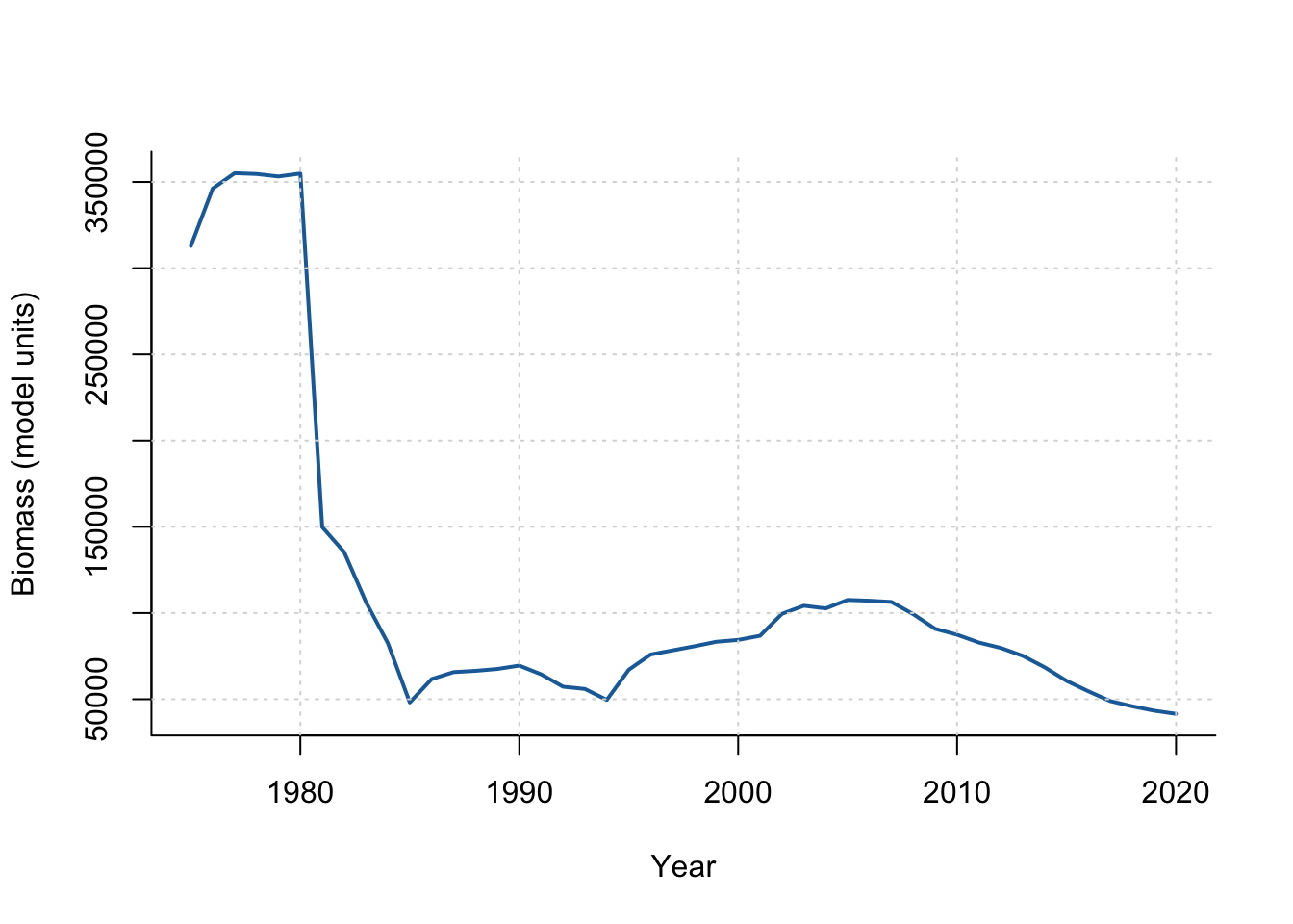

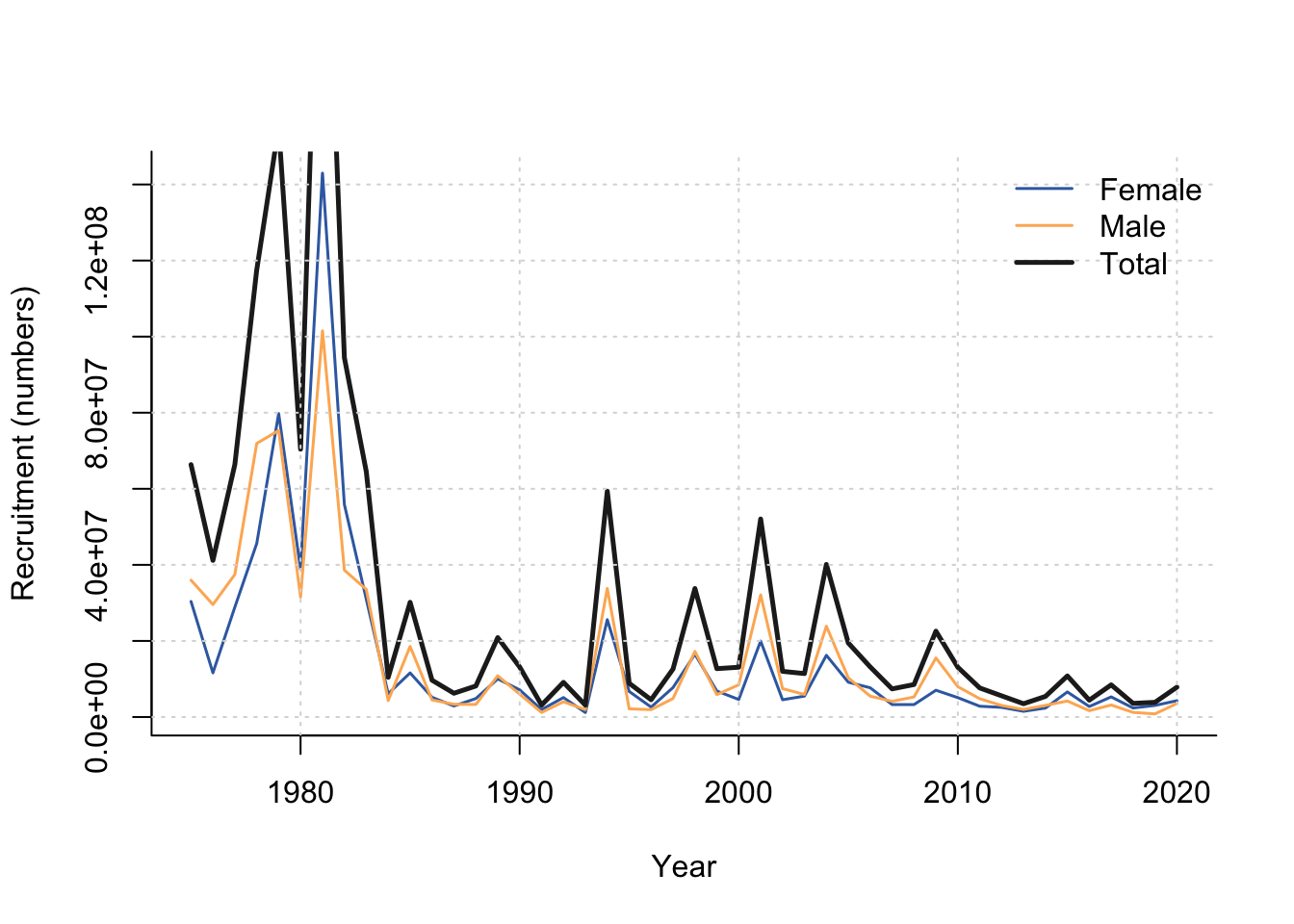
Figure 1: BBRKC biomass trajectory from the current RTMB population state.

Recruitment

Recruitment is summarized by sex and in total from the ported GMACS recruitment block:

\[ R_y = \sum_s R_{s,y}. \]

recruits <- rtmb_model$recruits[, seq_len(n_years), drop = FALSE]
recruitment_total <- colSums(recruits)

matplot(
  years, t(recruits), type = "l", lty = 1, lwd = 1.5,
  col = c("#386cb0", "#fdb462"),
  xlab = "Year", ylab = "Recruitment (numbers)", bty = "l"
)
lines(years, recruitment_total, lwd = 2.5, col = "#222222")
grid(col = "grey85")
legend(
  "topright", bty = "n", lty = 1, lwd = c(1.5, 1.5, 2.5),
  col = c("#386cb0", "#fdb462", "#222222"),
  legend = c("Female", "Male", "Total")
)

Figure 2: BBRKC recruitment trajectory from the current RTMB recruitment block.

Natural Mortality

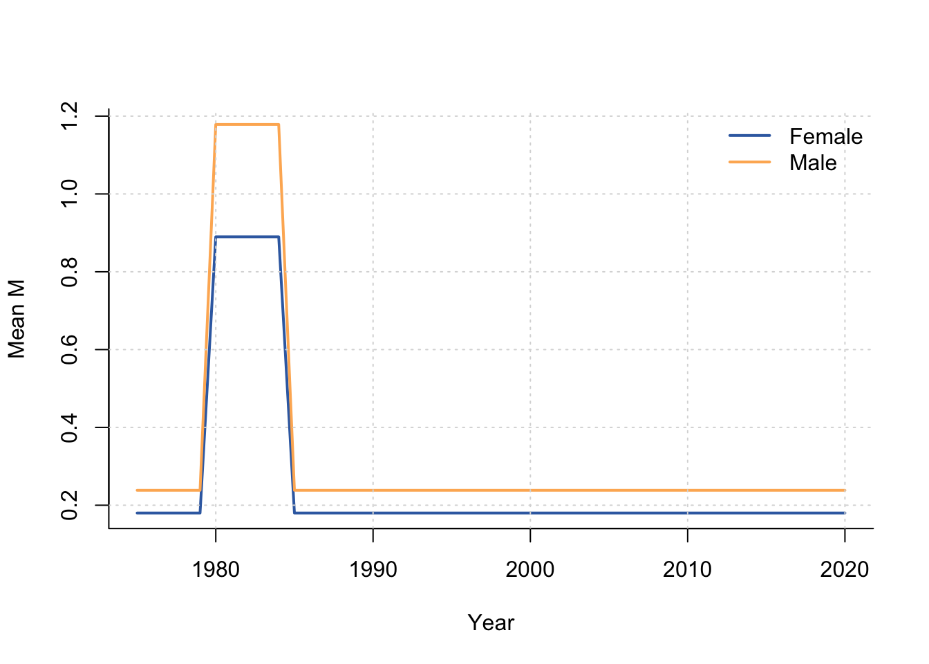
Natural mortality is plotted as an annual size-class mean by sex for the available mortality maturity stratum:

\[ \overline{M}_{s,y} = \frac{1}{L} \sum_\ell M_{s,m^*,y,\ell}. \]

n_sex <- rtmb_data$dimensions[["nsex"]]
maturity_index <- min(2L, dim(rtmb_model$M)[2])
mean_m <- matrix(NA_real_, nrow = n_years, ncol = n_sex)
for (sex in seq_len(n_sex)) {
  mean_m[, sex] <- rowMeans(rtmb_model$M[sex, maturity_index, seq_len(n_years), ])
}

matplot(
  years, mean_m, type = "l", lty = 1, lwd = 2,
  col = c("#386cb0", "#fdb462"),
  xlab = "Year", ylab = "Mean M", bty = "l"
)
grid(col = "grey85")
legend(
  "topright", bty = "n", lty = 1, lwd = 2,
  col = c("#386cb0", "#fdb462"),
  legend = c("Female", "Male")
)

Figure 3: Mean natural mortality by sex from the current RTMB mortality block.

Index Fit

Observed survey indices are plotted against the current RTMB predictions for each BBRKC index series.

index_fit <- index_fit_to_data_frame(rtmb_model, rtmb_data)
survey_obs <- rtmb_data$survey$data
index_fit$observed <- survey_obs$obs
series_ids <- sort(unique(index_fit$series))
panel_rows <- ceiling(length(series_ids) / 2)
panel_slots <- panel_rows * 2
old_par <- par(
  mar = c(3, 3, 2, 1),
  oma = c(0, 0, 0, 0)
)
layout(
  rbind(matrix(seq_len(panel_slots), ncol = 2, byrow = TRUE), rep(panel_slots + 1, 2)),
  heights = c(rep(1, panel_rows), 0.16)
)
for (series in series_ids) {
  x <- index_fit[index_fit$series == series, ]
  ylim <- range(c(x$observed, x$predicted), finite = TRUE)
  plot(x$year, x$observed, pch = 16, col = "#1b6da8", ylim = ylim,
       xlab = "", ylab = "", main = paste("Series", series), bty = "l")
  line_keys <- unique(x[c("fleet", "season", "sex", "maturity")])
  for (line_i in seq_len(nrow(line_keys))) {
    keep <- rep(TRUE, nrow(x))
    for (key_name in names(line_keys)) {
      keep <- keep & x[[key_name]] == line_keys[[key_name]][line_i]
    }
    line_x <- x[keep, ]
    line_x <- line_x[order(line_x$year), ]
    lines(line_x$year, line_x$predicted, lwd = 2, col = "#c43c39")
    points(line_x$year, line_x$predicted, pch = 1, col = "#c43c39")
  }
  grid(col = "grey88")
}
if (length(series_ids) < panel_slots) {
  for (unused in seq_len(panel_slots - length(series_ids))) {
    plot.new()
  }
}
par(mar = c(0, 0, 0, 0))
plot.new()
legend("center", horiz = TRUE, bty = "n",
       pch = c(16, NA), lty = c(NA, 1), lwd = c(NA, 2),
       col = c("#1b6da8", "#c43c39"), legend = c("Observed", "Predicted"))
layout(1)
par(old_par)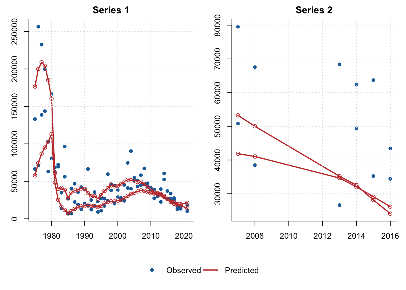

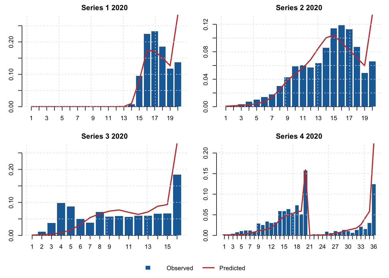
Figure 4: Observed and predicted BBRKC survey indices by series.

Size-Composition Fit

The panels below compare observed and predicted size compositions for recent rows from the first four modified composition series.

size_fit <- inputs$admb_size_fit
size_keys <- c("modified_series", "year", "fleet", "season", "sex", "type", "shell", "maturity")
size_key_rows <- unique(size_fit[size_fit$vector == "obs", size_keys])
size_key_rows <- size_key_rows[order(size_key_rows$modified_series, size_key_rows$year), ]
series_ids <- sort(unique(size_key_rows$modified_series))[1:4]
plot_records <- list()
for (series in series_ids) {
  candidates <- size_key_rows[size_key_rows$modified_series == series, ]
  key <- candidates[nrow(candidates), ]
  key_match <- rep(TRUE, nrow(size_fit))
  for (key_name in size_keys) {
    key_match <- key_match & size_fit[[key_name]] == key[[key_name]]
  }
  obs <- size_fit[key_match & size_fit$vector == "obs", c("size_bin", "value")]
  pred <- size_fit[key_match & size_fit$vector == "pred", c("size_bin", "value")]
  x <- merge(obs, pred, by = "size_bin", suffixes = c("_observed", "_predicted"))
  x <- x[order(x$size_bin), ]
  plot_records[[as.character(series)]] <- list(
    series = series,
    year = key$year,
    observed = x$value_observed / sum(x$value_observed),
    predicted = x$value_predicted / sum(x$value_predicted),
    size_bin = x$size_bin
  )
}
old_par <- par(mar = c(3, 3, 2, 1), oma = c(0, 0, 0, 0))
layout(rbind(matrix(1:4, ncol = 2, byrow = TRUE), c(5, 5)), heights = c(1, 1, 0.16))
for (rec in plot_records) {
  ylim <- range(c(rec$observed, rec$predicted), finite = TRUE)
  mids <- barplot(rec$observed, col = "#1b6da8", border = NA, ylim = ylim,
       xlab = "", ylab = "",
       main = paste("Series", rec$series, rec$year), bty = "l")
  axis(1, at = mids, labels = rec$size_bin)
  lines(mids, rec$predicted, lwd = 2, col = "#c43c39")
  grid(col = "grey88")
}
if (length(plot_records) < 4) {
  for (unused in seq_len(4 - length(plot_records))) {
    plot.new()
  }
}
par(mar = c(0, 0, 0, 0))
plot.new()
legend("center", horiz = TRUE, bty = "n",
       fill = c("#1b6da8", NA), border = c(NA, NA),
       lty = c(NA, 1), lwd = c(NA, 2), col = c(NA, "#c43c39"),
       legend = c("Observed", "Predicted"))
layout(1)
par(old_par)

Figure 5: Observed and predicted BBRKC size compositions for selected recent fit-summary rows.