Snow Crab GMACS Input and ADMB Fit Notes

Published

June 9, 2026

Purpose

This document is the Snow crab parallel to the BBRKC and Tanner pages. The Snow example in examples/snow includes GMACS input files plus ADMB output reports, so this page can summarize both parsed inputs and observed-vs-predicted ADMB fit diagnostics.

The current RTMB objective implementation is still BBRKC-specific. The Snow work here establishes parser coverage and report targets for a future Snow RTMB objective.

Files

File	Role
`examples/snow/gmacs.dat`	GMACS main run file.
`examples/snow/snow_21.dat`	Snow crab data file.
`examples/snow/snow_21.ctl`	Snow crab control file.
`examples/snow/snow_21.prj`	Snow crab projection file.
`examples/snow/gmacs.pin`	Fitted parameter state.
`examples/snow/Gmacsall.out`	ADMB likelihood and fit-summary output.
`examples/snow/gmacs.rep`	ADMB report output.

Reader

Code

source("R/read_gmacs_bbrkc.R")
source("R/gmacs_rtmb_nll.R")
source("R/read_gmacs_snow.R")

snow <- read_snow_inputs("examples/snow")
validate_snow_inputs(snow)

Input Summary

Code

dims <- snow$data$dimensions
data.frame(
  quantity = names(dims),
  value = as.integer(dims),
  row.names = NULL
)

  quantity value
1      syr  1982
2      nyr  2020
3  nseason     3
4   nfleet     8
5     nsex     2
6   nshell     1
7  nmature     2
8   nclass    22

Code

data.frame(
  component = c("catch", "survey", "size composition"),
  rows = c(
    sum(snow$data$catch$rows),
    nrow(snow$data$survey$data),
    sum(snow$data$size_comp$rows)
  )
)

         component rows
1            catch  156
2           survey   86
3 size composition  318

ADMB Report Summary

Code

snow_likelihood_summary(snow)

         block entries         sum
1     nloglike      32 -25907.3191
2  nlogPenalty      13    386.0459
3 priorDensity     655    487.2527

Code

data.frame(
  block = c("catch fit", "index fit", "size fit", "overall summary"),
  rows = c(
    nrow(snow$admb_catch_fit),
    nrow(snow$admb_index_fit),
    nrow(snow$admb_size_fit),
    nrow(snow$admb_overall_summary)
  )
)

            block  rows
1       catch fit   156
2       index fit    86
3        size fit 13992
4 overall summary    39

Index Fit

Observed survey indices are plotted against ADMB predicted values by series.

Code

index_fit <- snow$admb_index_fit
series_ids <- sort(unique(index_fit$series))
panel_rows <- ceiling(length(series_ids) / 2)
panel_slots <- panel_rows * 2
old_par <- par(mar = c(3, 3, 2, 1), oma = c(0, 0, 0, 0))
layout(
  rbind(matrix(seq_len(panel_slots), ncol = 2, byrow = TRUE), rep(panel_slots + 1, 2)),
  heights = c(rep(1, panel_rows), 0.16)
)
for (series in series_ids) {
  x <- index_fit[index_fit$series == series, ]
  ylim <- range(c(x$obs, x$predicted), finite = TRUE)
  plot(x$year, x$obs, pch = 16, col = "#1b6da8", ylim = ylim,
       xlab = "", ylab = "", main = paste("Series", series), bty = "l")
  line_keys <- unique(x[c("fleet", "season", "sex", "maturity")])
  for (line_i in seq_len(nrow(line_keys))) {
    keep <- rep(TRUE, nrow(x))
    for (key_name in names(line_keys)) {
      keep <- keep & x[[key_name]] == line_keys[[key_name]][line_i]
    }
    line_x <- x[keep, ]
    line_x <- line_x[order(line_x$year), ]
    lines(line_x$year, line_x$predicted, lwd = 2, col = "#c43c39")
    points(line_x$year, line_x$predicted, pch = 1, col = "#c43c39")
  }
  grid(col = "grey88")
}
if (length(series_ids) < panel_slots) {
  for (unused in seq_len(panel_slots - length(series_ids))) {
    plot.new()
  }
}
par(mar = c(0, 0, 0, 0))
plot.new()
legend("center", horiz = TRUE, bty = "n",
       pch = c(16, NA), lty = c(NA, 1), lwd = c(NA, 2),
       col = c("#1b6da8", "#c43c39"), legend = c("Observed", "Predicted"))
layout(1)
par(old_par)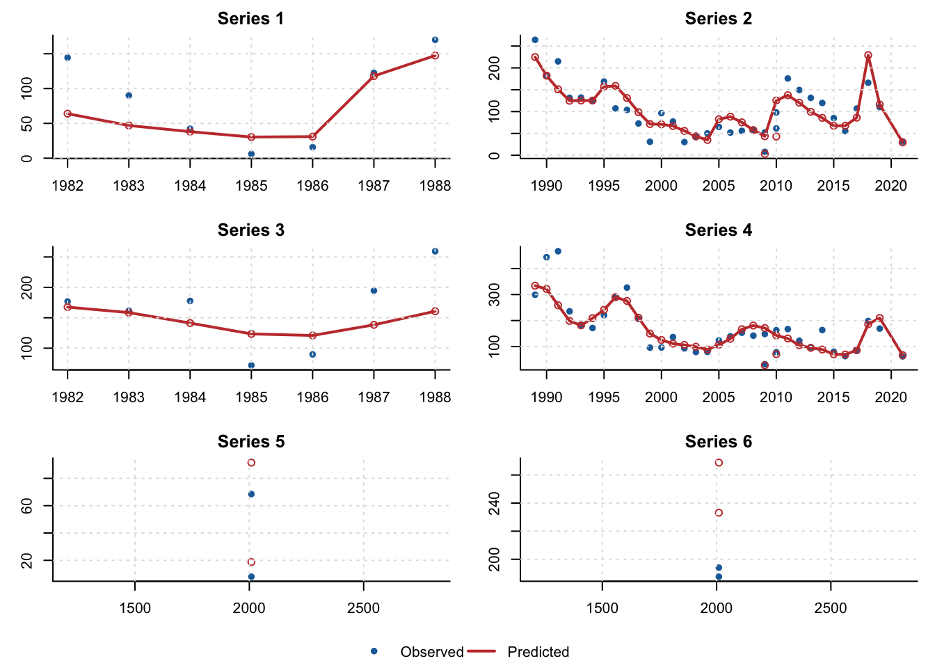

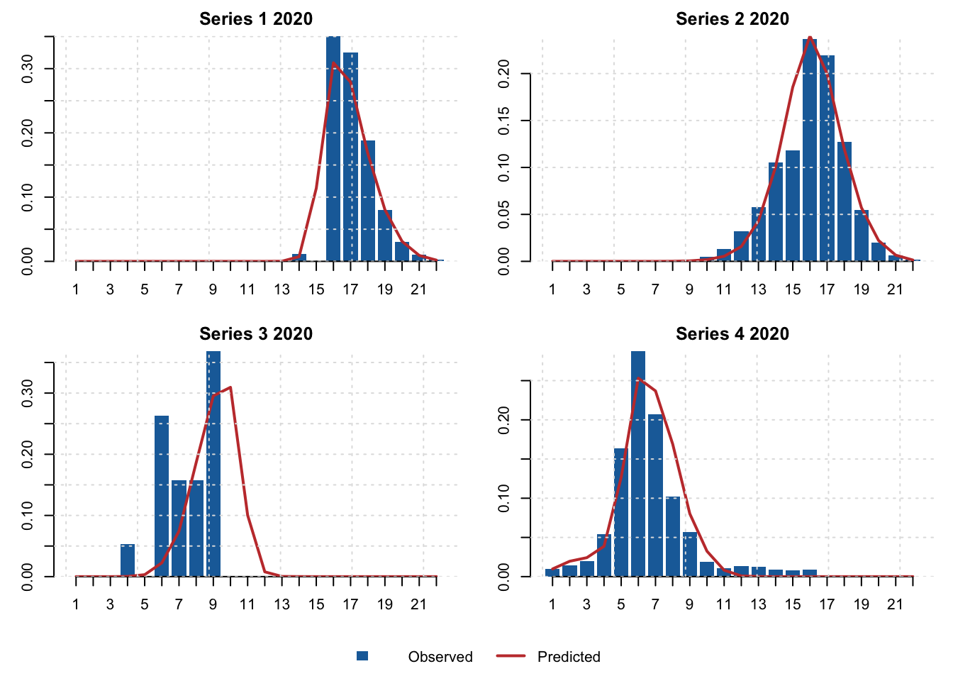
Figure 1: Observed and predicted Snow crab survey indices by series from ADMB output.

Size-Composition Fit

The panels below compare observed and predicted size compositions for recent rows from the first four modified composition series.

Code

size_fit <- snow$admb_size_fit
size_keys <- c("modified_series", "year", "fleet", "season", "sex", "type", "shell", "maturity")
size_key_rows <- unique(size_fit[size_fit$vector == "obs", size_keys])
size_key_rows <- size_key_rows[order(size_key_rows$modified_series, size_key_rows$year), ]
series_ids <- sort(unique(size_key_rows$modified_series))[1:4]
old_par <- par(mar = c(3, 3, 2, 1), oma = c(0, 0, 0, 0))
layout(rbind(matrix(1:4, ncol = 2, byrow = TRUE), c(5, 5)), heights = c(1, 1, 0.16))
for (series in series_ids) {
  candidates <- size_key_rows[size_key_rows$modified_series == series, ]
  key <- candidates[nrow(candidates), ]
  key_match <- rep(TRUE, nrow(size_fit))
  for (key_name in size_keys) {
    key_match <- key_match & size_fit[[key_name]] == key[[key_name]]
  }
  obs <- size_fit[key_match & size_fit$vector == "obs", c("size_bin", "value")]
  pred <- size_fit[key_match & size_fit$vector == "pred", c("size_bin", "value")]
  x <- merge(obs, pred, by = "size_bin", suffixes = c("_observed", "_predicted"))
  x <- x[order(x$size_bin), ]
  observed <- x$value_observed / sum(x$value_observed)
  predicted <- x$value_predicted / sum(x$value_predicted)
  ylim <- range(c(observed, predicted), finite = TRUE)
  mids <- barplot(observed, col = "#1b6da8", border = NA,
       ylim = ylim, xlab = "", ylab = "",
       main = paste("Series", series, key$year), bty = "l")
  axis(1, at = mids, labels = x$size_bin)
  lines(mids, predicted, lwd = 2, col = "#c43c39")
  grid(col = "grey88")
}
if (length(series_ids) < 4) {
  for (unused in seq_len(4 - length(series_ids))) {
    plot.new()
  }
}
par(mar = c(0, 0, 0, 0))
plot.new()
legend("center", horiz = TRUE, bty = "n",
       fill = c("#1b6da8", NA), border = c(NA, NA),
       lty = c(NA, 1), lwd = c(NA, 2), col = c(NA, "#c43c39"),
       legend = c("Observed", "Predicted"))
layout(1)
par(old_par)

Figure 2: Observed and predicted Snow crab size compositions for selected recent rows.