
Overview
afscOSA is an R library that produces one step ahead (OSA) residual diagnostic plots for composition data fit in fisheries stock assessments at the Alaska Fisheries Science Center (AFSC). OSA residuals are computed using the compResidual R library (Trijoulet and Nielsen, 2022; Trijoulet et al., 2023). OSA residuals are available in afscOSA for composition data fit assuming a multinomial or Dirichlet-multinomial distribution from purely fixed effects assessment models.
For each data set (i.e., fleet), the output includes plots of the fit to aggregate compositions across years, a Q-Q plot of OSA residuals, and bubble plots for OSA and Pearson residuals. OSA residuals will be standard normal under a correctly specified model and so statistics are also provided to give context to the fit and guide understanding of causes of misfit. See Stewart and Monnahan (2025) for information on background and interpretation.
Installation
afscOSA relies on the compResidual R library. Install both using the instructions below:
# see https://github.com/fishfollower/compResidual#composition-residuals for more detailed
# installation instructions

TMB:::install.contrib("https://github.com/vtrijoulet/OSA_multivariate_dists/archive/main.zip")
remotes::install_github("fishfollower/compResidual/compResidual", force=TRUE)

remotes::install_github("noaa-afsc/afscOSA", force=TRUE)
Example: OSAs as a Diagnostic for Model Misspecification
In the example below, we demonstrate how OSA residuals detect common stock assessment model misspecifications in age composition data. We simulate 30 years of composition data under three scenarios using a logistic selectivity baseline:
- Correctly Specified Model: The expected proportions and effective sample size () match the underlying data-generating process.
- Misspecified : The model assumes double the true effective sample size ( vs. true ), overestimating data precision.
- Misspecified Selectivity: The model assumes logistic selectivity, but the true underlying process follows dome-shaped selectivity.
We calculate the OSA residuals with run_osa() and compare the diagnostic output using plot_osa(). To ensure bubble sizes remain visually consistent across different stock assessments and fleet comparisons, plot_osa() caps maximum bubble sizes at 6 and issues a warning listing any truncated values:
library(afscOSA)

nbins <- 10 # age bins
Neff <- 50  # multinomial sample size
nyrs <- 30 # really no. of replicates for now
e1 <- matrix(rep(plogis(seq(-10,10, len=nbins)), times=nyrs),
             ncol=nbins, byrow=TRUE)

## Simulate data
set.seed(1233)
# correctly specified
o1 <- t(apply(e1, 1, function(x) rmultinom(1, Neff, x)))
# wrong Neff (Neff too big; i.e., the model assumes the data is twice as precise
# as it actually is)
o2 <- t(apply(e1, 1, function(x) rmultinom(1, floor(Neff/2), x)))
# mispecified selex: change underlying selectivity shape from logistic to dome-shape
ewrong <- e1
ewrong[,(nbins-2):nbins] <- ewrong[,(nbins-2):nbins]/2
o3 <- t(apply(ewrong, 1, function(x) rmultinom(1, Neff, x)))

x1 <- run_osa(obs=o1, exp=e1, N=rep(Neff, nyrs), fleet='Correct', index=1:nbins,
             index_label = 'age', years=1:nyrs, seed=10)
x2 <- run_osa(obs=o2, exp=e1, N=rep(Neff, nyrs), fleet='Misspecified Neff', index=1:nbins,
              index_label = 'age', years=1:nyrs, seed=10)
x3 <- run_osa(obs=o3, exp=e1, N=rep(Neff, nyrs), fleet='Misspecified Selex', index=1:nbins,
              index_label = 'age', years=1:nyrs, seed=10)

plot_osa(list(x1, x2, x3), use_agg_proportions = FALSE)
#> Warning in plot_osa(list(x1, x2, x3), use_agg_proportions = FALSE): The
#> following Pearson residuals were set to 6 for plotting: 6.25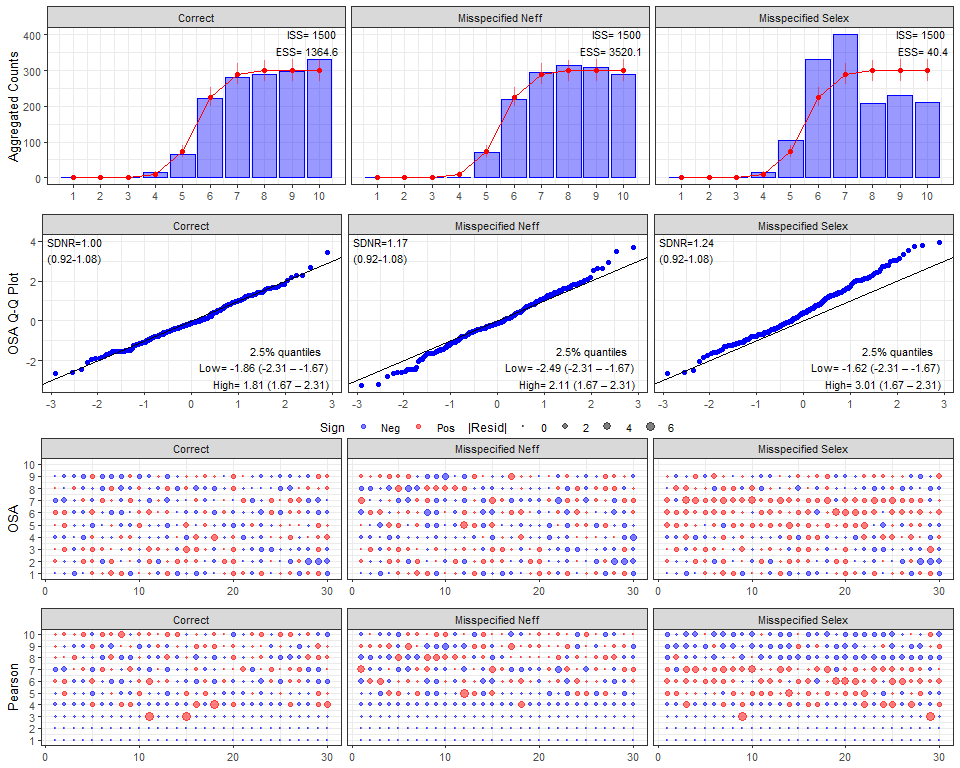
Interpretation and use of diagnostics
The function plot_osa provides a set of tools that can be used for statistical model validation, i.e., gauging whether the composition data reasonably came from the fitted assessment model. These tools can be used to identify when misfit occurs and give clues about how the model could be modified to better fit the data. The package follows the advice and guidance of Stewart and Monnahan (2025) for composition data specifically, and Kapur et al. (2025)’s recommendations to examine multiple diagnostics, use caution when using standalone diagnostics for selecting a “best” model, and avoid a strict reliance of rejecting models based on p-values. Specifically, a model fit with a statistically significant misfit (e.g., a value outside the confidence interval) should not be rejected outright. Instead, the visual and statistical tools provided here are intended to give context to model fit and provide a consistent framework for reporting it for AFSC assessments.
The top plot of the output shows the fits to each bin aggregated over all years (histogram). For a given model the model expectation (red points) and aggregate sample size (ISS=input sample size, ESS=effective sample size) define a new aggregate distribution which can be used to calculate the 95% percentiles of data expected from each bin (red vertical bars). Note that these are not confidence intervals because they show the spread of data and are not Bayesian posterior predictive intervals because they ignore parameter uncertainty. They simply represent what kind of data would be expected from the model for a given bin, and observations that lie well outside an interval suggest misfit. The y-axis can be set to counts to visually show the relative differences among sample sizes of different fleets, or as proportions (the default). This aggregate fit will identify systematic misfit as caused typically by the wrong selectivity form. Since the model should typically get this right it is shown at the top and considered the first validation tool to examine. However, systematic misfit across cohorts or only for some time periods may not be visible in these plots.
In the simulated example above the aggregate fits are good for the first two columns but clearly is mispecified for the last. Aggregate fits do not detect the wrong sample size (data weighting). The ESS on the second column provides the first hint that something is amiss.
The next plot is the quantile-quantile (Q-Q) plot of the OSA residuals (blue points). Under a correctly specified model these should be standard normal and thus fall along the 1:1 line. Two statistics are presented: the standard deviation of the normalized residuals (SDNR) which should be 1, and the lower and upper 2.5% percentiles of the residuals. All three statistics also show the 95% confidence interval by default but these can be disabled. These statistics depend on the sample size (number of residuals) so that a departure from expected is case specific. The main advantage of OSA residuals is that their distribution is known under a correctly specified model and so deviations away from this suggest misfit of some kind, whether the visual fit or the statistics measuring the SD or tail properties. It is important to note that the power to detect misfit may be low given sample sizes frequently seen in stock assessments.
The SDNR and tail quantiles are within the confidence intervals for the first column, suggesting no evidence for misfit as expected. The two misspecified models have SDNR values higher than expected and poor tail quantities and suggest serious misfit exists. After using OSA statistics to conclude likely misfit, the cause for both cases is apparent from the aggregate plots: the wrong sample size and misspecified selectivity, respectively.
The Q-Q plot often will suggest that misfit exists but not what aspect of the model is misspecified. Bubble plots of the residuals can be used to look for temporal or other patterns that can hint at the causes of misfit. Pearson residual bubble plots have long been used and thus are familiar and easy to interpret for most analysts. The downside of the Pearson residuals is that it is unclear what their distribution is under a correctly specified model. OSA bubble plots are thus also shown, however their calculation depends on bin order and the terminal bin has no residuals and so they can be difficult to interpret. Together the OSA and Pearson bubble plots can help analysts identify issues with misfit, particularly time blocks or cohort issues. These two bubble plots have the same bubble size among panels within a fleet and among fleets. Residuals larger than 6 are truncated (with a console warning) to help with visualization.
The bubble plots are not needed to identify causes of misfit in these examples. However, it is instructive to examine the OSA residuals for the two misspecified models since the misspecification is known in these cases. In particular notice the large Pearson residuals in the correctly specified case. Pearson residuals >6 are expected for this model.
References
Kapur, M. S., N. Ducharme-Barth, M. Oshima, and F. Carvalho. 2025. Good practices, trade-offs, and precautions for model diagnostics in integrated stock assessments. Fisheries Research 281:107206.
Stewart, I. J. and C. C. Monnahan (2025). “Diagnosing common sources of lack of fit to composition data in fisheries stock assessment models using one-step-ahead (OSA) residuals.” Canadian Journal of Fisheries and Aquatic Sciences 82: 1-13. 10.1139/cjfas-2025-0158
Trijoulet, V., Nielsen, A. 2022. compResidual: Residual calculation for compositional observations. R package version 0.0.1.
Trijoulet, V., Albertsen, C.M., Kristensen, K., Legault, C.M., Miller, T.J. and Nielsen, A., 2023. Model validation for compositional data in stock assessment models: calculating residuals with correct properties. Fisheries Research, 257, p.106487.