
Refinements to Rceattle for eastern Bering Sea pollock
Rceattle working paper for the 2024 assessment configuration
Abstract
The custom AD Model Builder (ADMB) stock assessment model developed for eastern Bering Sea walleye pollock has a long history of application. For a variety of reasons, including general recommendations from the 2025 Center for Independent Experts (CIE) reviews, the custom ADMB code has been successfully ported to R Template Model Builder (RTMB). That conversion provides access to advanced RTMB features and makes the underlying code easier to understand and modify. Similarly, adopting more generic platforms, such as Rceattle, can provide access to more modern software developments. In this study, we tailored Rceattle code and configurations so that Rceattle can closely mimic the custom ADMB/RTMB assessment code. The Rceattle configuration uses the supported multinomial composition likelihood with a robustifying constant and a non-parametric selectivity form. We also evaluated a two-dimensional, first-order autoregressive (AR1) selectivity sensitivity; it did not converge and remains a research topic. An exploratory dynamic structural equation modeling (DSEM) analysis shows how recruitment covariates can be compared by cohort, separately from the final assessment configuration.
NoteAI-assisted development
Artificial intelligence (AI) tools were used to aid document development and model implementation. AI-assisted material was reviewed and revised by the authors, who retain responsibility for the scientific content, code, analyses, interpretations, and conclusions.

Rceattle WORKING PAPER
Download a PDF version of this report
1 Executive Summary
Building from the ADMB-to-RTMB conversion, this analysis evaluates whether Rceattle can be configured to reproduce the main features of the 2024 eastern Bering Sea pollock “PM” assessment while providing a model that is easier to extend. This update focuses on the Rceattle configuration, comparison with the modified ADMB model, model diagnostics, and projection inputs.
When the Rceattle parameters and fishery selectivity are set to the same values used in the ADMB model, Rceattle reproduces numbers-at-age, spawning biomass, and predicted catch to numerical precision. Mean absolute differences are 0.000117% for spawning biomass and 0.000143% for predicted catch. This result establishes agreement in the population dynamics when both implementations use the same parameter values.
When Rceattle was fit to the data, the convergence criteria were fully met, including a positive-definite Hessian. The least-identified direction remained in annual ATS/AVO selectivity deviations, but the added direct coefficient-increment penalty reduced the condition number below the warning threshold. Relative to the ADMB fit, mean absolute differences were 1.5% for spawning biomass, 0.7% for recruitment, and 10.3% for total biomass. These small differences are concentrated in the earliest years; the remaining uncertainty is primarily estimability of the annual selectivity deviations.
The 2D age-by-year AR1 selectivity sensitivity was included as an initial diagnostic attempt. Results appeared broadly similar to the non-parametric constrained selectivity fits. However, because some parameters reached bounds, the model failed to converge. Closer examination of this selectivity form will continue as a research topic.
One-step-ahead residuals and nine terminal-year-consistent retrospective peels have been generated from the Rceattle configuration. Aggregate composition residual dispersion is lower than the standard-normal reference. Mohn’s rho is 0.261 for spawning biomass, 0.119 for total biomass, 0.147 for recruitment, and -0.077 for fishing mortality. Forty-eight of 50 jitters returned to the best solution; two found a substantially poorer mode. These results focus subsequent work on selectivity identification, retrospective bias, and observation-model sensitivity.
2 Purpose and Scope
The September 2026 review focuses on whether the Rceattle configuration has sufficient documentation for Plan Team evaluation. This working paper serves that focused purpose rather than the broader purpose of a full Stock Assessment and Fishery Evaluation (SAFE) chapter.
This working paper therefore records:
- what was run from those development files;
- how the Rceattle outputs compare with the modified ADMB reference;
- which diagnostics are available now;
- which sensitivities remain research-only; and
- what work would help structure the next evaluation pass.
The report uses the Alaska Stock Assessment Report (asar) package for glossary conventions and accessibility guidance (Schiano et al. 2026). Those practices helped prepare the Quarto source for Section 508 review, including semantic headings and tables, descriptive figure captions, and alternative text. They support accessibility but do not replace final manual and agency-approved compliance checks.
Standard SAFE report sections such as background material, fishery history, ecosystem narrative, reference-point tables, and harvest advice are outside the scope of this document. Projection calculations are included only to test the export and use of the Rceattle results.
3 Rceattle Configuration
3.1 Model Inputs
The Rceattle configuration uses the prepared workbook Data/EBS_24_pollock_m23_rceattle_full_1964-2024.xlsx. The data builder retains every age from 1 through 15. Fishery compositions use nominal sample sizes; bottom trawl survey (BTS) and acoustic-trawl survey (ATS) sample sizes use the integer values aligned with the modified ADMB model. Age-1 survey selectivity remains separately parameterized from the age-2–15 curve, and each likelihood contribution evaluates the complete 15-age composition. Compositions use the multinomial likelihood with a robustifying constant. We added a constant of 0.001 to both observed and expected proportions before evaluating the likelihood. This prevents log(0) and limits the influence of observations in bins with expected proportions near zero.
The run uses Rceattle version 5.8.1 from upstream commit 7bb694788012, with the model configuration synchronized to Rceattle-models commit 3dc99ddfbf9e.
The next-assessment update script review is complete, and execution awaits complete new-year observations. The script duplicates terminal records and places placeholders for new catch, composition, and survey observations. The script serves as a template until complete new-year observations are available; after population, it creates a complete assessment workbook.
3.2 Selectivity
The configuration uses NonParametricPM fishery selectivity with annual deviations. When fit to the data, the model reached a small maximum gradient. The Hessian condition number was approximately 489,000 and the convergence criteria were fully met. Its least-identified direction remained concentrated in sel_coff_dev, specifically the shared ATS/AVO block rather than the shared fishery/CPUE block.
The time-varying selectivity penalties use explicit standard deviations on log-selectivity random-walk increments. The fishery and its shared CPUE selectivity block use an SD of 0.500, ATS and AVO use 0.138, and BTS uses 1.000. ATS and AVO also use a direct coefficient-increment penalty (Sel_curve_pen3 = 0.1) to constrain the across-age common-mode direction that is removed by annual selectivity normalization. The fishery specification also retains the ADMB-matched curve-shape penalty weights (12.5, 1/60, and 1) and an average-selectivity centering weight of 10. These values are penalty coefficients rather than SDs.
The fitting sequence, composition-likelihood sensitivity, and 2D age-by-year AR1 development work are documented in the appendix.
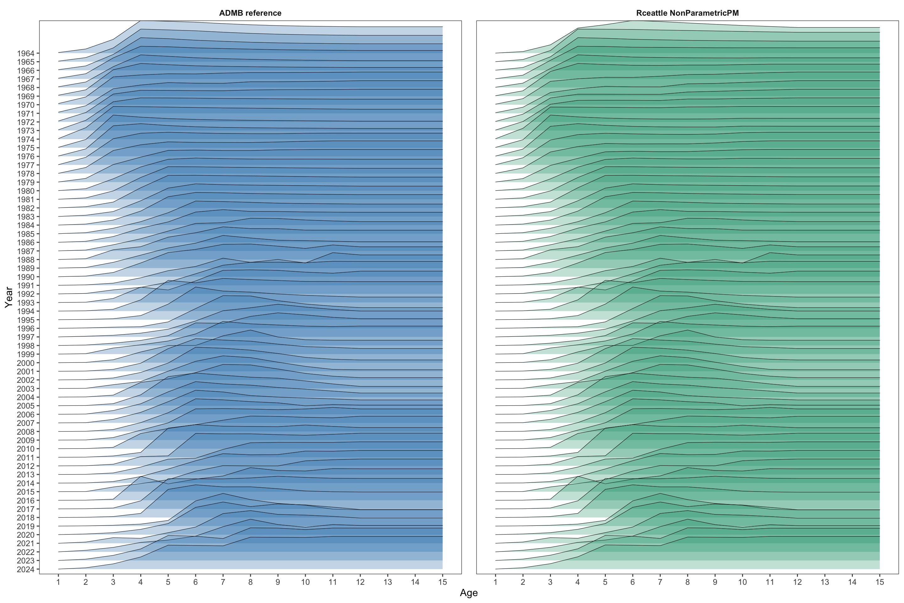
The ADMB and Rceattle fishery selectivity curves have similar age patterns, while their annual variation differs most in the earlier years (Figure 1).
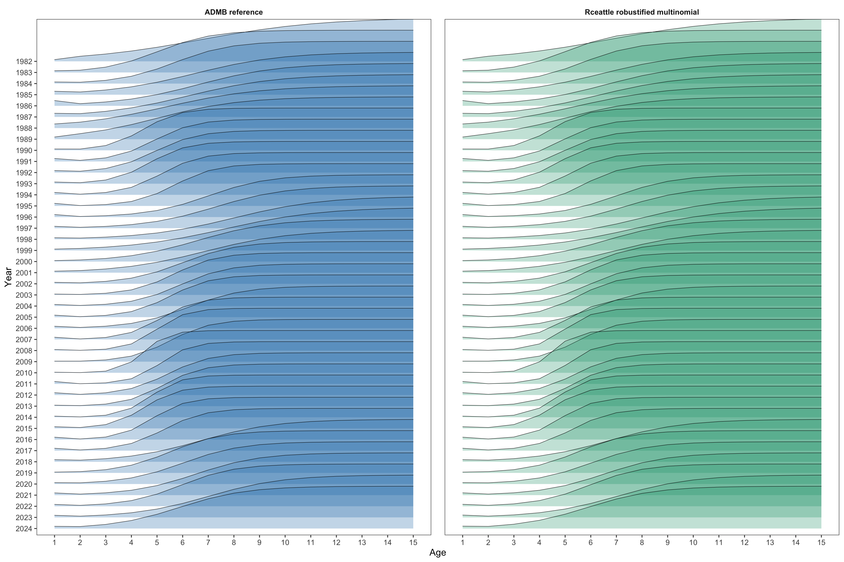
For the BTS, both implementations use a logistic selectivity curve for ages 2–15 and override age 1 with a separately estimated parameter. The age-1 term therefore does not lie on the fitted logistic curve. Its annual deviation is multiplicative on the age-1 log-selectivity parameter, and the CV on the year-to-year deviations is specified at 25%. Rceattle encodes this ADMB specification as LogisticPM; the plotted age-1 values are the realized annual selectivities after applying the separate parameter and its annual deviations.
The BTS age compositions contribute directly to estimation of this selectivity through the multinomial likelihood with a robustifying constant. For each of the 42 BTS composition years, predicted numbers at age are formed from population abundance at the survey timing, BTS selectivity at age, and the ageing-error matrix, and are then normalized across ages 1–15. Catchability cancels during this normalization, so the compositions primarily inform the age pattern of selectivity and the population age structure rather than the absolute survey scale. In particular, the observed age-1 proportion informs the separate age-1 selectivity parameter and its annual deviations; ages 2–15 inform the logistic slope, inflection, their annual deviations, and abundance at age.
For year \(y\), the fitted contribution is
\[ -w_y N_y \sum_{a=1}^{15}(o_{y,a}+c) \log\left(\frac{p_{y,a}+c}{o_{y,a}+c}\right), \]
where \(o_{y,a}\) and \(p_{y,a}\) are observed and predicted proportions, \(c=0.001\), and the fleet composition weight \(w_y\) is 1. The nominal BTS sample sizes are truncated to the integer values read by ADMB; they range from 48 to 329 and sum to 5,403 across years. No young- or old-tail accumulation is used, so age 1 remains in the likelihood as its own bin. Larger-\(N_y\) years exert more influence, while \(c\) stabilizes empty or near-empty bins. The composition contributions are optimized jointly with the BTS biomass index likelihood and the selectivity random-walk penalties; the fitted curve therefore balances annual age-composition fit, survey biomass fit, and temporal smoothness. Both implementations preserve the distinct age-1 term outside the logistic ages 2–15 curve (Figure 2).
4 ADMB Comparison Results
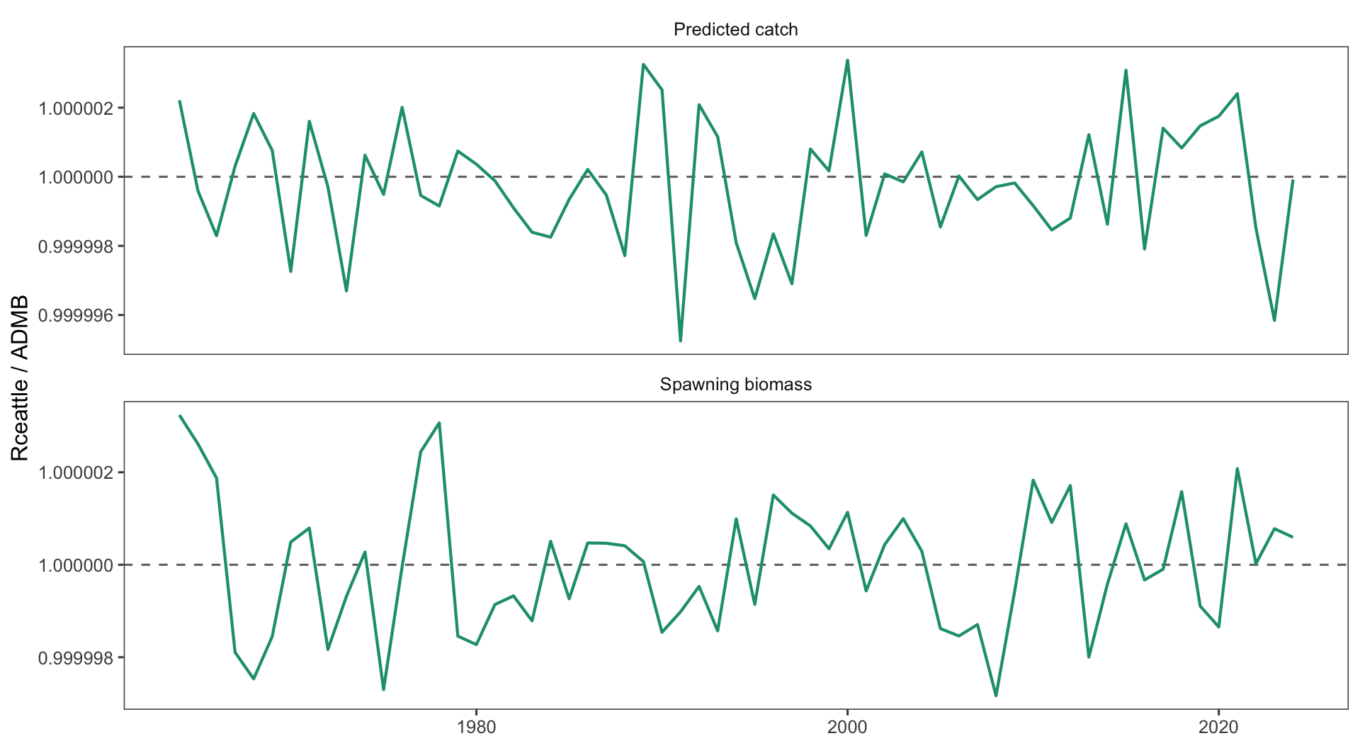
When the Rceattle parameters and fishery selectivity are set to the ADMB values, the two programs give nearly identical population calculations. Mean absolute differences are 0.000117% for spawning biomass and 0.000143% for predicted catch. Annual Rceattle-to-ADMB ratios for both quantities remain extremely close to one (Figure 3).
The reported Rceattle likelihood contributions are 140.191 for indices, -123.761 for catch, 3572.874 for age compositions, and 98.379 for recruitment deviations. Their sum is 3704.588. The ADMB tot_like and dat_like values are 736.724 and 459.931, respectively, but cannot be compared directly because the two programs include different likelihood terms, penalties, and constants. The ADMB maximum absolute gradient is 3.47e-04; no Rceattle model-parameter gradient is available from this comparison because Rceattle does not estimate parameters in this run.
| Quantity | Correlation | Mean absolute (%) | Maximum absolute (%) | 2024 difference (%) |
|---|---|---|---|---|
| Rceattle configuration | ||||
| Recruitment | 1.00 | 0.70 | 8.21 | −4.97 |
| Spawning biomass | 1.00 | 1.45 | 9.96 | 2.88 |
| Total biomass | 0.98 | 10.32 | 95.63 | 2.61 |
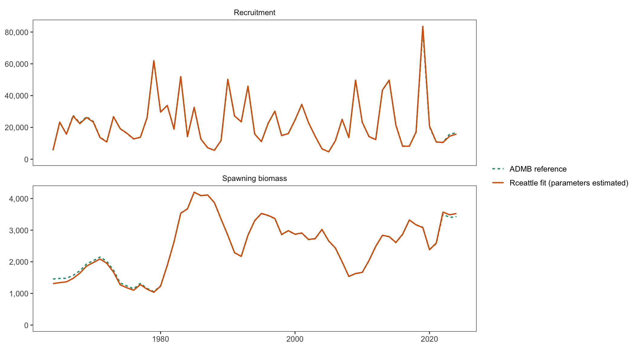
When Rceattle estimates its parameters, the fitted trajectories differ most from ADMB during the early period and in the terminal recruitment estimate (Figure 4). These trajectories are distinct from the run in which Rceattle parameters are set to the ADMB values. The fitted trajectories remain highly correlated with the ADMB reference, with relatively small mean annual differences (Table 1). Development sensitivities are documented in the appendix.
The Rceattle fit has a small maximum gradient and a positive-definite Hessian. Adding the direct ATS/AVO coefficient-increment penalty reduced the condition number from approximately 1.14 million to 489,000 and removed the prior Hessian-conditioning warning. The residual weakest direction remains almost entirely in the shared time-varying ATS/AVO selectivity coefficients, not the fishery/CPUE coefficients, so this block remains an appropriate focus for sensitivity checks even though the formal warning is resolved.
5 Diagnostics
The fitted Rceattle model fully met the convergence criteria: it reached a small maximum gradient, had a positive-definite Hessian, and remained below the Hessian-condition-number warning threshold. The supporting diagnostic products include OSA residuals, retrospectives, self-tests, and jitter tests (Table 2).
| Diagnostic | Current status | Review use |
|---|---|---|
| ADMB-parameter comparison | Completed and saved in the ADMB-to-Rceattle comparison outputs. | Primary numerical agreement check. |
| Rceattle fit | Convergence criteria were fully met, with a positive-definite Hessian and a condition number of approximately 489,000. | Primary Rceattle comparison fit to the data. |
| OSA residuals | Completed for 1,864 residuals and saved in RDS outputs. | Useful, but analytical and exactly reproduced index groups need interpretation. |
| Rceattle retrospectives | Nine peels completed and fully met the convergence criteria. | The revised peels preserve data availability and fix terminal fishery/CPUE selectivity increments at zero, holding the terminal selectivity-at-age curve at its preceding-year value. |
| Legacy ADMB retrospectives | Existing ADMB retro.rep files are present. | Provides historical context distinct from the Rceattle retrospective peels. |
| Rceattle 5.8.1 self-tests | Fifty initial-start and 50 estimated-start refits fully met the convergence criteria. | Supports the revised positive-index simulation workflow; it does not resolve observed-data multimodality. |
| Jitter tests | Forty-eight of 50 jitters returned to the best mode; two WARN fits reached an inferior mode. | Documents multimodality in the observed-data fit. |
5.1 Rceattle 5.8.1 self-test validation
Rceattle 5.8.1 changed simulation of natural-scale normal and multivariate normal survey indices. The fitted likelihood remains an untruncated normal; the simulator redraws non-positive values because data_check() excludes them. The resulting self-test therefore uses a normal distribution truncated at zero whenever rejection occurs.
The ADMB-to-Rceattle comparison was rerun first with Rceattle 5.8.1. Its saved summary gives mean absolute differences of 0.000117% for spawning biomass and 0.000143% for predicted catch. This confirms that the package update preserved the agreement in the population calculations.
The self-test uses the same delivered EBS workbook and supported multinomial criterion with the same robustifying constant as the Rceattle configuration. The observed-data fit reproduced the stored objective of 716.948070 and maximum gradient of 0.000041; the convergence criteria were fully met, including a positive-definite Hessian. The Hessian condition number was approximately \(4.9 \times 10^5\); its least-identified direction remained concentrated in the shared ATS/AVO sel_coff_dev block rather than fishery/CPUE.
| Metric | Value |
|---|---|
| Initial-start self-tests converged | 5.000000e+01 |
| Estimated-start self-tests converged | 5.000000e+01 |
| Paired fits with objective difference greater than 0.0001 | 0.00000e+00 |
| Maximum absolute paired objective difference | 3.09564e-08 |
| Median across-simulation median SSB percent bias | -1.055% |
| Median terminal-year SSB percent bias | -0.907% |
| Fleets with at least one row above 2 percent rejection probability | 2.00000e+00 |
| Maximum row-level non-positive probability | 6.66814e-02 |
All 50 phased simulations fully met the convergence criteria when refitted from the original initial values. Repeating the same simulated datasets from the fitted parameter values also produced 50 fits that fully met the criteria. Paired objectives agreed within \(3.1 \times 10^{-8}\), so these simulations showed no start-dependent mode. Median spawning-biomass bias was -1.06% across years and -0.91% in the terminal year. These results validate the revised self-test workflow; they do not rule out the mode previously encountered when fitting the observed data (Table 3).
| Fleet | Code | Distribution | Rows | Maximum row probability | Mean row probability | Rows above 2% |
|---|---|---|---|---|---|---|
| ATS | 4 | Lognormal | 19 | 0.00% | 0.00% | 0 |
| ATS_1 | 6 | Lognormal | 18 | 0.00% | 0.00% | 0 |
| AVO | 2 | Normal | 18 | 3.88% | 0.23% | 1 |
| BTS | 3 | MVN | 42 | 6.64% | 0.17% | 1 |
| BTS_1 | 5 | Lognormal | 42 | 0.00% | 0.00% | 0 |
| CPUE | 7 | Normal | 12 | 0.00% | 0.00% | 0 |
One AVO row had a 3.76% non-positive probability and one BTS multivariate-normal row had a 6.67% probability. Those rows exceed the package’s 2% warning threshold and should be identified when interpreting recovery. CPUE and the remaining index series had negligible or zero marginal rejection probability (Table 4).
5.2 OSA Residuals
OSA residuals run on the Rceattle configuration. The aggregate composition fits are generally close, while all three OSA quantile plots are narrower than the standard-normal reference (Figure 5). These diagnostics apply to the fitted NonParametricPM selectivity configuration. The failed 2D-AR1 sensitivity and ADMB-to-Rceattle calculation use separate results. The composition diagnostics use afscOSA version 0.0.1 and pass Rceattle’s internally calculated residuals to afscOSA::run_osa(). The residual builder uses complete ages 1–15, with nominal fishery sample sizes and the integer BTS and ATS sample sizes aligned with the modified ADMB model. This follows the current afscOSA interpretation guidance while retaining Rceattle’s residual calculation.
Following that guidance, the aggregate age-composition fits are the first check for systematic misfit, including patterns that could indicate an unsuitable selectivity form. The red vertical ranges contain 95% of data simulated from the fitted multinomial model conditional on the aggregate sample size and estimated parameter values held constant. They represent conditional simulation variability. The quantile–quantile plots then assess whether the OSA residuals resemble a standard normal distribution. The standard deviation of normalized residuals (SDNR) should be near one, and the displayed tail statistics provide a separate check on extreme residual behavior. Finally, the OSA and Pearson bubble plots are used to look for age, year, or cohort patterns that may suggest the source of misfit. Each statistic and nominal interval contributes to an integrated diagnostic interpretation rather than an automatic model-rejection rule.
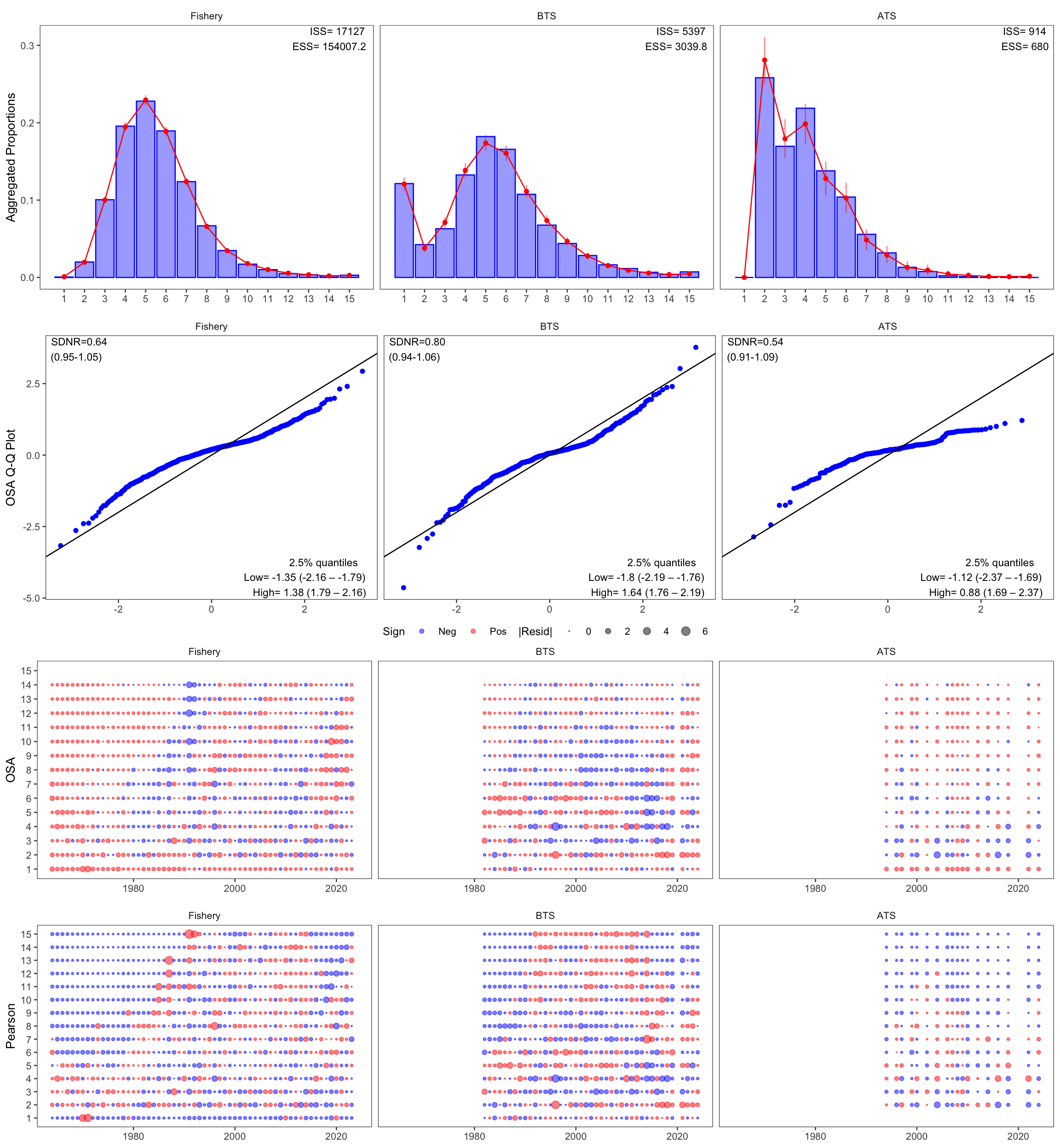
The aggregate observed and fitted compositions are generally close, although the survey panels contain some age-specific departures. The OSA distributions are narrower than the standard-normal reference for all three composition sources: SDNR is 0.64 for the fishery, 0.80 for BTS, and 0.53 for ATS. Their tail diagnostics also show shorter-than-expected tails. Together these results indicate underdispersion relative to the fitted multinomial observation model. Model selection requires this information alongside the full suite of diagnostics. The bubble plots should instead be used to identify persistent age, year, or cohort patterns and to guide focused checks of selectivity, composition weighting, and observation-model assumptions. One Pearson residual (8.86) is capped at 6 in the figure, following the package’s plotting convention.
5.3 Retrospective patterns
Nine retrospective peels were run from the Rceattle fit. The unpeeled model ends in 2024, and the peeled fits end in 2023 through 2015. Each peel preserves the data-availability pattern of the 2024 model. Thus, fishery age compositions end one year before the peel terminal year, survey series retain their historical sampling schedule and terminal lags, and earlier discontinued series retain their original ending years.
Each peel applies the fitting sequence documented in the appendix. The terminal-year fishery and mirrored catch-per-unit-effort selectivity increments are fixed at zero. All nine final fits fully met the convergence criteria, with maximum gradients from 2.1e-05 to 6.4e-05.
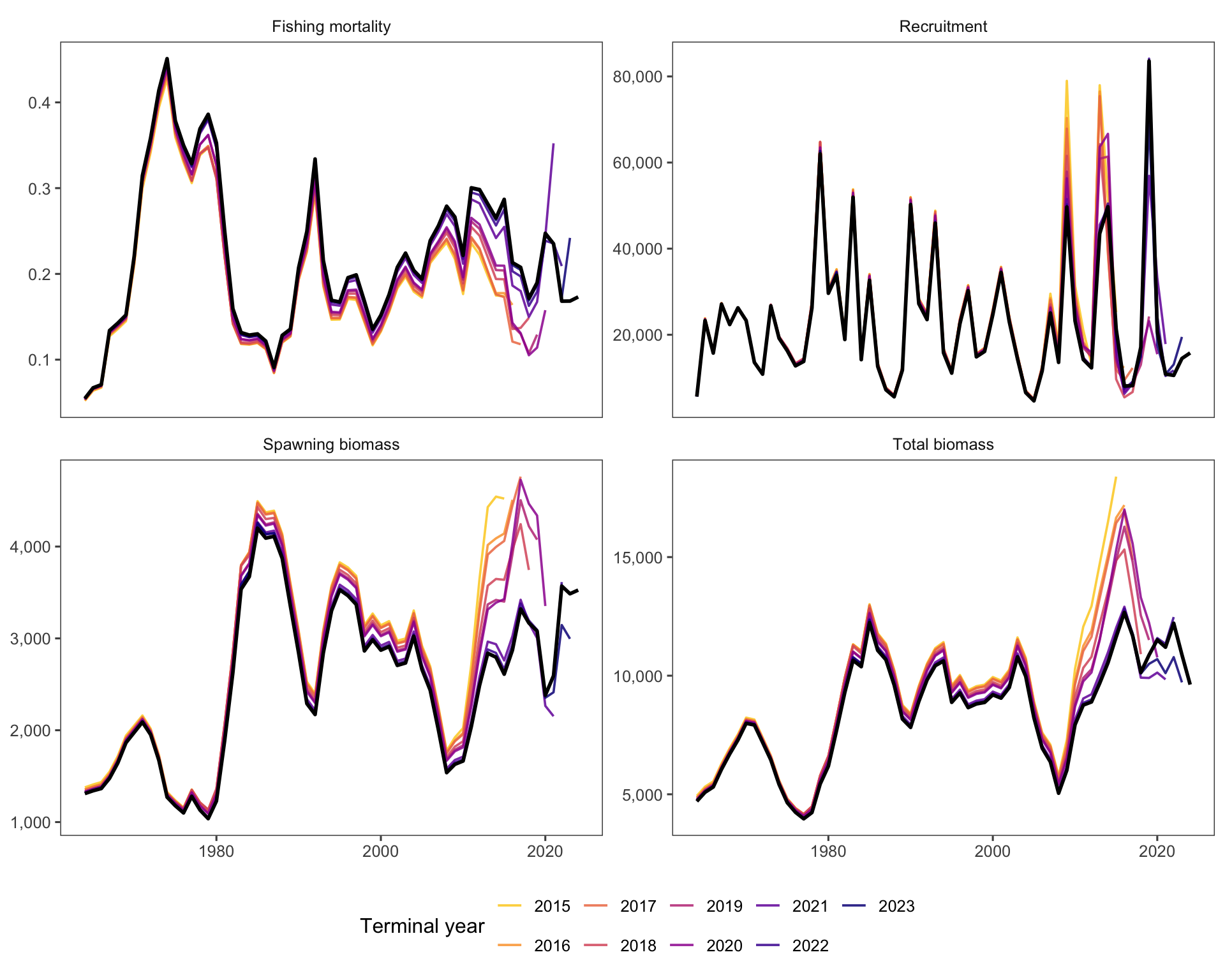
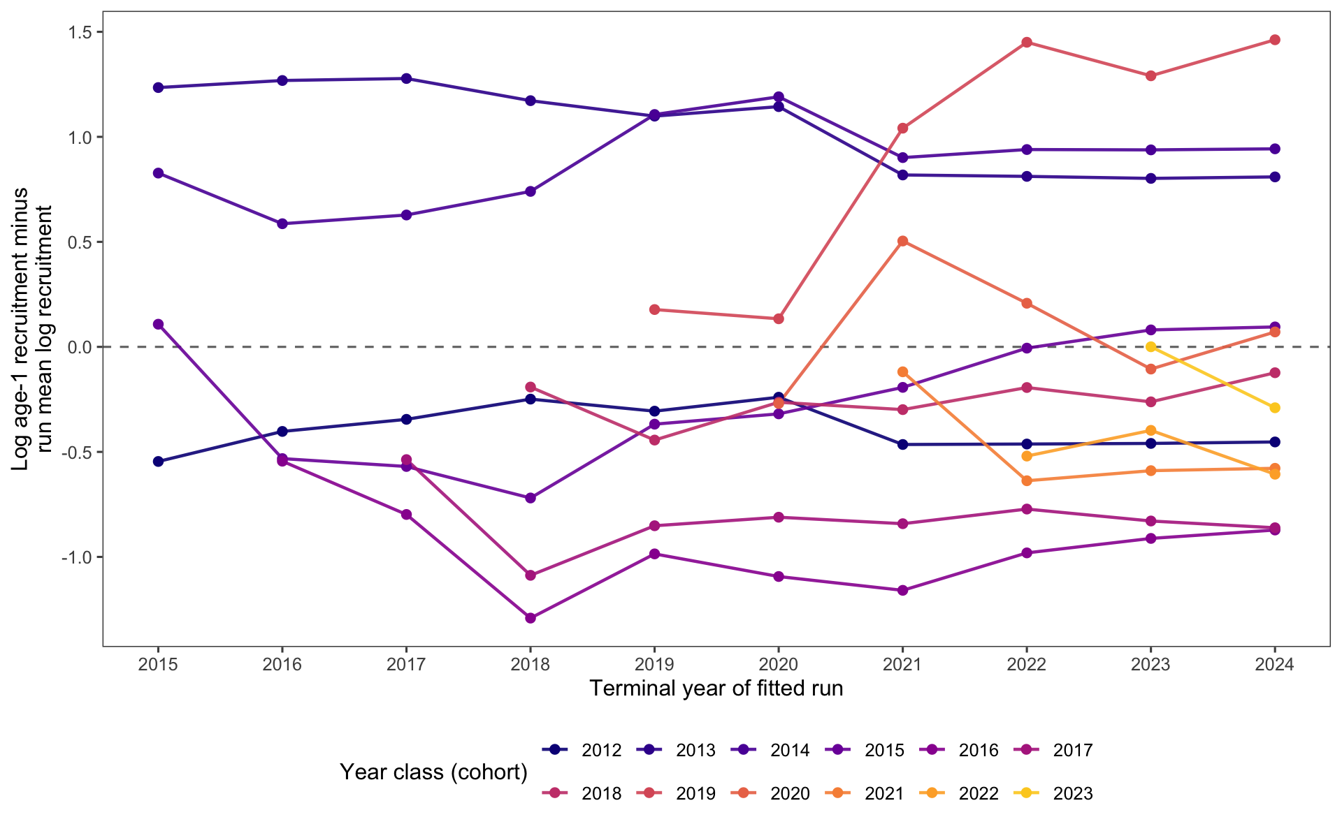
The NonParametricPM fishery selectivity is parameterized at age. The base sel_coff parameters and annual sel_coff_dev random-walk increments apply to age bins; the fishery uses 12 estimated bins and holds older ages at the last estimated value. Fixing every terminal-year increment at zero therefore holds the realized terminal selectivity-at-age curve at the preceding-year curve. Across all peels and both the fishery and mirrored catch-per-unit-effort series, the maximum absolute terminal-to-preceding-year difference was 8.9e-16. These Rceattle fits are separate from the legacy AD Model Builder (ADMB) retrospective files. The model runs with earlier terminal years generally estimate greater spawning biomass and recruitment and lower fishing mortality over their shared years (Figure 6). Cohort-specific revisions to age-1 recruitment are isolated in Figure 7. Within each fitted run, the plotted values are log age-1 recruitment centered by that run’s mean log recruitment over 1978 through its terminal year. Zero therefore represents the run-specific geometric mean rather than zero recruitment.
| Quantity | Peels | Mohn's rho |
|---|---|---|
| Total biomass | 9 | 0.119 |
| Spawning biomass | 9 | 0.261 |
| Recruitment | 9 | 0.147 |
| Fishing mortality | 9 | −0.077 |
The estimated Mohn’s rho values are 0.261 for spawning biomass, 0.119 for total biomass, 0.147 for recruitment, and -0.077 for fishing mortality. Across the recent nine-year period, the available data and model tended to overestimate recruitment and spawning biomass when recent years of data were successively removed. Fishing mortality showed the opposite pattern, with lower estimates when recent data were removed. Spawning biomass shows the largest average relative difference. The fully met convergence criteria and small gradients support interpretation of these values as properties of the revised retrospective specification, while the magnitude of spawning-biomass rho motivates continued evaluation of selectivity, survey influence, and recent recruitment estimates (Table 5).
5.3.1 Cohort revision and data-source diagnostics
The elevated spawning biomass in model runs with terminal years set to 2015–2020 is associated primarily with the initially large estimates of the 2013 and 2014 year classes, with a smaller contribution from the 2012 year class. Those cohorts support much of the estimated spawning biomass during 2015–2020 as they recruit to the mature population. The purpose of the following diagnostics is to learn which data signals and model processes cause their estimated strength, and consequently spawning biomass, to shift downward when later observations are included. For example, between model runs with terminal years set to 2020 and 2021, estimated age-1 abundance declines from 63,618 to 45,548 million fish for the 2013 cohort and from 66,666 to 49,473 million fish for the 2014 cohort. The corresponding estimate for the 2012 cohort declines from 15,947 to 12,622 million fish.
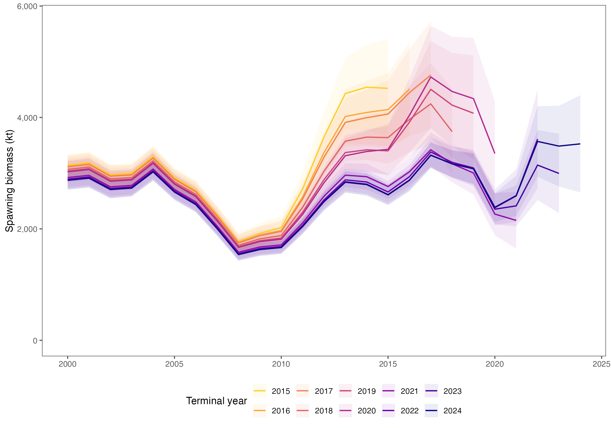
This uncertainty display is directly comparable in intent to the historical ADMB retrospective figure supplied for reference. Both show the same broad qualitative feature: earlier terminal-year fits produce higher spawning biomass over the mid-2010s, but with substantial uncertainty. The comparison does not establish identical causes because the ADMB and Rceattle retrospectives differ in implementation and fitted configuration. The Rceattle bands also represent approximate, conditional Hessian uncertainty; they should not be interpreted as uncertainty in the retrospective bias itself (Figure 8).
The transition from the 2020 to 2021 peel is especially informative because it contains the main downward step. Five records become available: the 2020 fishery age composition (effective sample size 565.2), the 2021 BTS biomass index (4,889 kt), the 2021 BTS age composition (effective sample size 149), the 2021 AVO index, and the BTS age-1 index record. Controlled refits began at the converged all-data 2021 solution and used the same parameter map. Each refit removed one newly available observation block, so these results measure conditional influence rather than providing independent alternative models.
The survey context makes this transition unusual. NOAA Fisheries canceled the 2020 eastern Bering Sea bottom-trawl survey, along with the standard vessel-based pollock acoustic survey, because the COVID-19 pandemic prevented safe survey operations (NOAA Fisheries 2020). The missing BTS observation therefore created a two-year interval between the 2019 and 2021 BTS biomass estimates. AFSC used three saildrone uncrewed surface vehicles to collect acoustic observations across the standard pollock survey area as a substitute for the research-vessel acoustic sampling. That effort provided useful abundance information, but it lacked the trawl samples used to identify species and estimate the age and size composition of the acoustic signal. NOAA consequently characterized the information as less detailed and more uncertain than a standard vessel survey, and the assessment assigned the estimate greater observation error (NOAA Fisheries 2020). This combination of a missing BTS year and a higher-uncertainty acoustic substitute reduces the continuity of fishery-independent information available to track the 2012–2014 cohorts before the 2021 BTS observation enters.
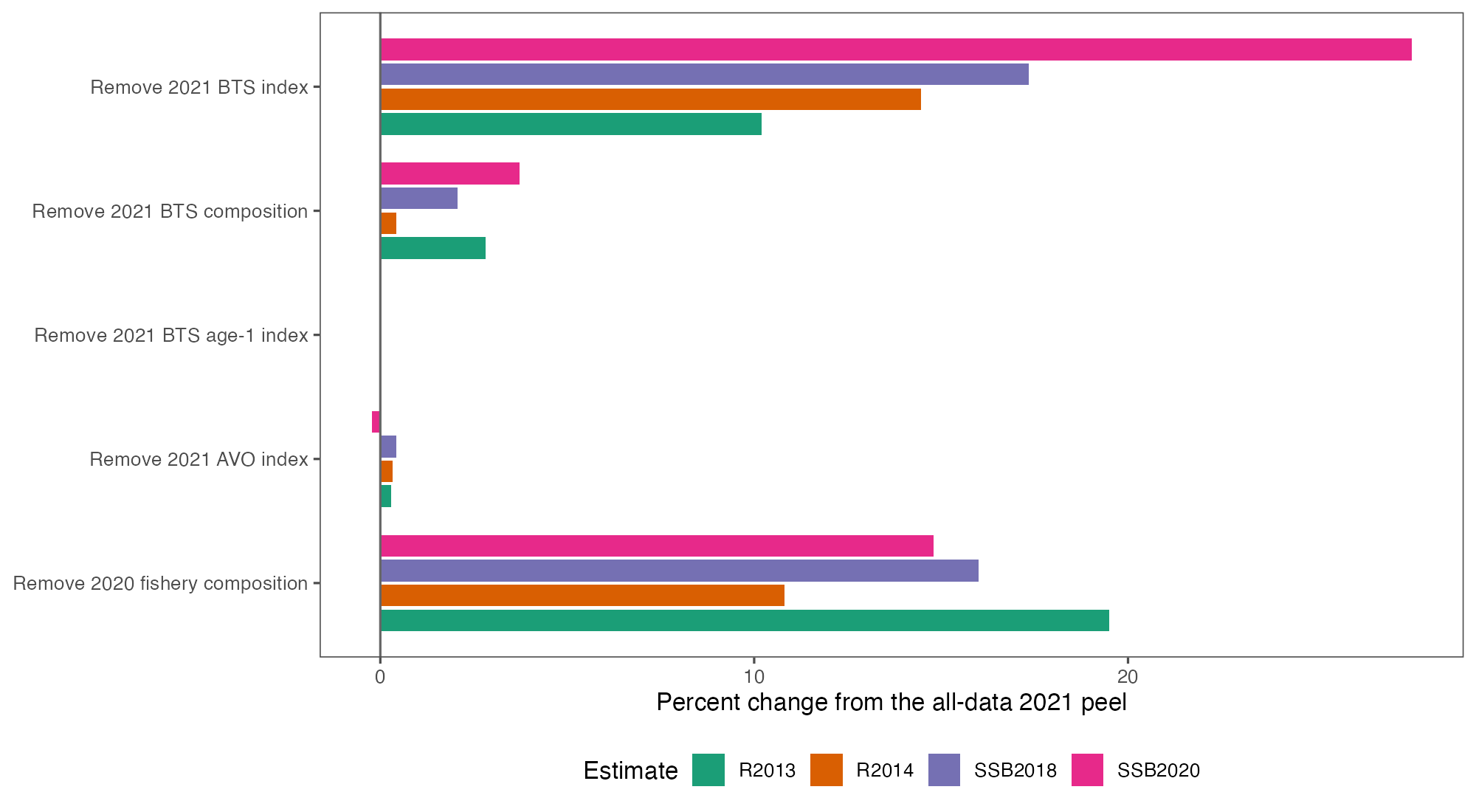
Removing the 2021 BTS biomass index increases the 2013 and 2014 recruitment estimates by 10.2% and 14.5%, respectively, and increases 2020 spawning biomass by 27.6%. Removing the 2020 fishery age composition increases the two cohort estimates by 19.5% and 10.8% and 2020 spawning biomass by 14.8%. In contrast, removing the 2021 BTS age composition changes these quantities by only about 0–4%, removing AVO changes them by less than 0.5%, and removing the BTS age-1 index has no effect on these older cohorts. The cumulative addition experiment gives the same ordering: adding the 2020 fishery composition produces the first major decline, adding the 2021 BTS index produces the second, and the BTS composition and AVO index make smaller subsequent adjustments (Figure 9; Table 6).
| Scenario | R2013 (%) | R2014 (%) | SSB 2018 (%) | SSB 2020 (%) | Maximum gradient |
|---|---|---|---|---|---|
| 2020 data availability | 39.8 | 29.5 | 38.9 | 44.7 | 4.68 × 10⁻⁵ |
| Add 2020 fishery composition | 10.0 | 10.5 | 14.1 | 25.1 | 1.07 × 10⁻⁴ |
| Add 2021 BTS index | 3.1 | 0.7 | 2.4 | 3.6 | 4.28 × 10⁻⁵ |
| Add 2021 BTS composition | 0.3 | 0.3 | 0.4 | −0.2 | 4.59 × 10⁻⁵ |
| Add 2021 AVO index | 0.0 | 0.0 | 0.0 | 0.0 | 4.43 × 10⁻⁵ |
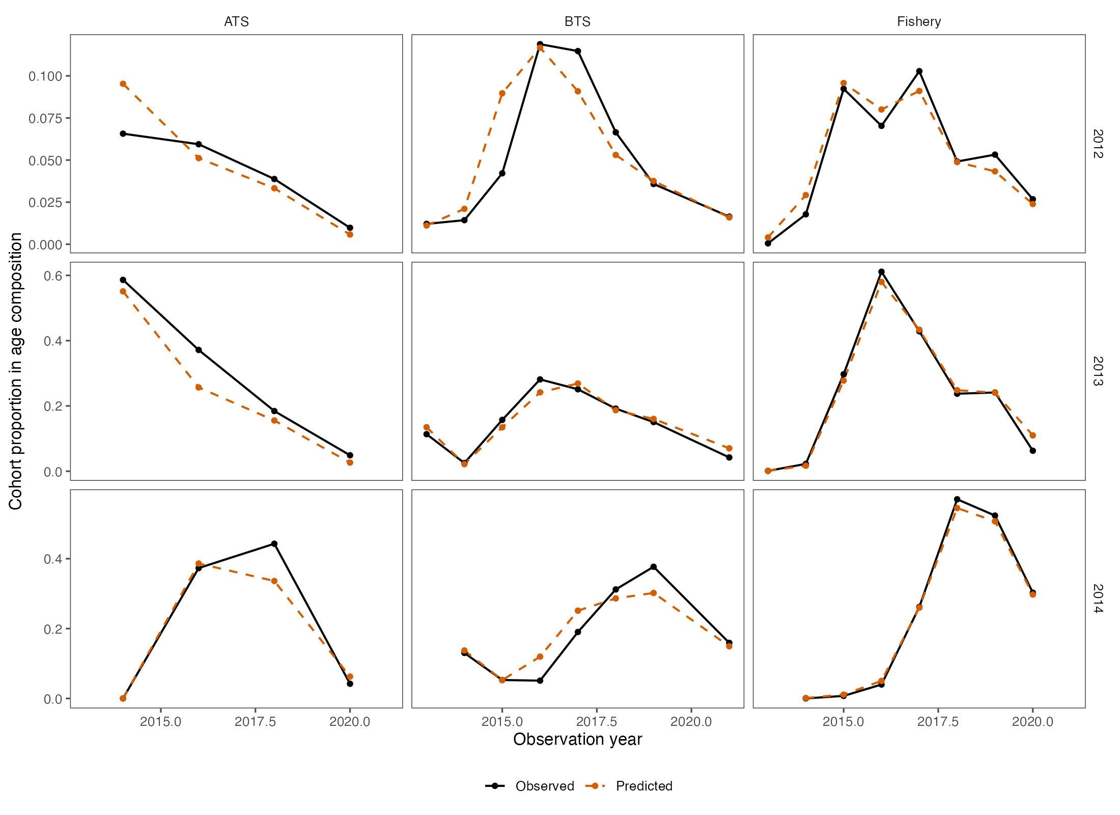
The composition traces clarify why the fishery record is influential. For the 2013 cohort at age 8, the 2020 fishery observed proportion is 0.063 compared with a fitted proportion of 0.110. The 2021 BTS composition also places less mass on that cohort at age 9 (0.042 observed versus 0.070 fitted), but its conditional leverage is smaller. Evidence for the 2014 cohort is less uniform: its fishery and BTS terminal proportions are close to their fitted values. The 2013 cohort therefore shows a recognizable late-age composition signal across two data sources, whereas the 2014 downward revision is tied more strongly to the overall BTS abundance scale and the model’s allocation of that abundance among ages (Figure 10).
Selectivity is an important mediator rather than a separate observation. When the 2021 peel is refit with BTS selectivity fixed at its realized 2020-peel curves, the 2013 and 2014 recruitment estimates increase by 14.5% and 14.9%, and 2020 spawning biomass increases by 19.2%, relative to the all-data 2021 fit. Fixing fishery and CPUE selectivity at their 2020-peel curves has much smaller and mixed effects. Thus, the lower 2021 BTS index supplies the main new abundance-scale information, and re-estimated BTS selectivity determines how much of that scale change is assigned to these cohorts (Table 7).
| Scenario | R2013 (%) | R2014 (%) | SSB 2018 (%) | SSB 2020 (%) | Maximum gradient |
|---|---|---|---|---|---|
| All selectivity re-estimated | 0.0 | 0.0 | 0.0 | 0.0 | 4.43 × 10⁻⁵ |
| Fishery and CPUE fixed at 2020 peel | 3.1 | −4.0 | −4.9 | −4.7 | 1.06 × 10⁻⁴ |
| BTS fixed at 2020 peel | 14.5 | 14.9 | 19.9 | 19.2 | 3.43 × 10⁻⁵ |
These experiments narrow the source of the shift but do not yet identify a unique biological process. Natural mortality is fixed in this configuration, so the model cannot represent cohort-specific anomalous survival directly. The same observations could instead reflect changing survey availability or movement, ageing or composition inconsistencies, or selectivity changes that are not fully separated from abundance. The next diagnostic stage should therefore (1) audit the age determinations and sample construction for the 2013 cohort in the 2020 fishery and 2021 BTS samples, (2) map the spatial and size composition of the 2019 and 2021 BTS observations to test availability changes across the survey gap, (3) profile or otherwise perturb BTS selectivity while retaining the 2021 index, and (4) run a targeted cohort-survival or time-varying-mortality sensitivity. Until those checks are complete, the evidence supports a data-conflict/selectivity explanation for the downward revision, not a definitive attribution to mortality or any single survey record.
6 Projections
The projections carry the terminal Rceattle population state and biological schedules forward under the seven Tier 3 harvest alternatives implemented in the Standard Projection Model (J. Ianelli 2026). Fishery selectivity and fishing mortality represent average conditions during 2020–2024. All alternatives use the same assessment results and fixed catches for 2025 and 2026, after which their harvest rules produce different catch, biomass, and fishing-mortality trajectories. The technical conversion, execution steps, and validation checks are documented in Appendix A-2.
| spmR Projection Files | ||
|---|---|---|
| file | role | exists |
| spm.dat | SPM setup | TRUE |
| pm.prj | Rceattle-derived species input | TRUE |
| tacpar.dat | TAC parameters | TRUE |
| spm | SPM executable | TRUE |
| age_schedules.csv | Rceattle-derived age schedules | TRUE |
| fishery_selectivity_recent_years.csv | Annual fishery selectivity used in the recent-year average | TRUE |
The saved projection products include the population inputs, projection controls, simulation output, and summary tables used in this section (Table 8).
| Generated SPM Setup and Source Information | |
|---|---|
| Item | Value |
| Rceattle source fit | nonparametric_pm |
| Composition likelihood | Multinomial with c = 0.001 |
| Composition sample sizes | fishery nominal; BTS and ATS integer sample sizes aligned with modified ADMB |
| spmR version | 0.3.0 |
| Terminal assessment year | 2024 |
| Fishery selectivity rule | arithmetic mean of annual selectivity-at-age |
| Fishery selectivity years | 2020, 2021, 2022, 2023, 2024 |
| Recent average-F years | 2020, 2021, 2022, 2023, 2024 |
| Spawning timing | 0.25 year from January 1 (start of April) |
| Rceattle encoding | spawn_month = 3 elapsed months; 3/12 = 0.25 |
| SPM encoding | Spawnmo = 4 as a one-based calendar-month code; (4 - 1)/12 = 0.25 |
| Timing compatibility check | Matched: both calculations apply survival through 0.25 of the year |
| Spawning-biomass timing convention | Mature spawning biomass after survival through 0.25 of the year: N × exp(-0.25 Z) × maturity × spawning weight |
| Projection begin year | 2025 |
| Projection years | 14 |
| Simulations | 1000 |
| Alternatives | 1, 2, 3, 4, 5, 6, 7 |
The projection setup identifies the assessment source, biological timing, averaging years, simulation count, and harvest alternatives (Table 9).
| SPM Projection Alternatives | ||
|---|---|---|
| Alternative | Name | Description |
| 1 | Maximum permissible ABC | Maximum permissible Tier 3 ABC harvest rate. |
| 2 | Author-specified ABC | Author-specified adjustment to the Tier 3 ABC harvest rate; the current multiplier is 1.0. |
| 3 | Average recent F | Recent average fishing mortality from the Rceattle-derived input file. |
| 4 | Alternative SPR rate | User-specified SPR rate of 0.60. |
| 5 | No fishing | Zero fishing mortality after the fixed-catch years. |
| 6 | OFL threshold determination | OFL harvest rate for threshold and status-determination calculations. |
| 7 | Status-determination ramp | Maximum permissible ABC for three years followed by the OFL status-determination calculation. |
The seven alternatives span maximum permissible ABC, recent fishing mortality, a higher spawning-potential-ratio target, no fishing, and status-determination calculations (Table 10).
6.1 Seven Tier 3 Scenario Results
Catches for 2025 and 2026 are fixed at 1,350 thousand t in every alternative; the alternatives therefore first diverge in 2027 (Table 11). The reported values are simulation means from 1,000 SPM simulations.
| Seven Tier 3 Projection Alternatives | ||||||||
|---|---|---|---|---|---|---|---|---|
| Alt | Scenario | Year | Catch | ABC | OFL | SSB | F | B/B35 |
| 1 | Maximum permissible ABC | 2027 | 1,864 | 1,864 | 2,259 | 2,476 | 0.350 | 1.17 |
| 1 | Maximum permissible ABC | 2028 | 1,308 | 1,308 | 1,583 | 2,115 | 0.310 | 1.00 |
| 2 | Author-specified ABC | 2027 | 1,864 | 1,864 | 2,259 | 2,476 | 0.350 | 1.17 |
| 2 | Author-specified ABC | 2028 | 1,308 | 1,308 | 1,583 | 2,115 | 0.310 | 1.00 |
| 3 | Average recent F | 2027 | 1,132 | 1,132 | 2,259 | 2,582 | 0.200 | 1.22 |
| 3 | Average recent F | 2028 | 1,015 | 1,015 | 1,963 | 2,446 | 0.200 | 1.16 |
| 4 | Alternative SPR rate | 2027 | 856 | 856 | 2,259 | 2,619 | 0.150 | 1.24 |
| 4 | Alternative SPR rate | 2028 | 803 | 803 | 2,103 | 2,585 | 0.150 | 1.22 |
| 5 | No fishing | 2027 | 0 | 0 | 2,259 | 2,726 | 0.000 | 1.29 |
| 5 | No fishing | 2028 | 0 | 0 | 2,455 | 3,034 | 0.000 | 1.44 |
| 6 | OFL threshold determination | 2027 | 1,561 | 1,561 | 1,561 | 2,017 | 0.370 | 0.95 |
| 6 | OFL threshold determination | 2028 | 1,210 | 1,210 | 1,210 | 1,831 | 0.340 | 0.87 |
| 7 | Status-determination ramp | 2027 | 1,509 | 1,809 | 1,809 | 2,211 | 0.320 | 1.05 |
| 7 | Status-determination ramp | 2028 | 1,424 | 1,424 | 1,424 | 1,977 | 0.360 | 0.94 |
| Projection Age-Specific Schedules | |||||
|---|---|---|---|---|---|
| Age | Spawning_weight | Fishery_weight | Maturity | Natural_mortality | Selectivity |
| 1 | 0.085 | 0.025 | 0.000 | 0.900 | 0.000 |
| 2 | 0.196 | 0.186 | 0.008 | 0.450 | 0.061 |
| 3 | 0.322 | 0.401 | 0.289 | 0.300 | 0.220 |
| 4 | 0.534 | 0.667 | 0.641 | 0.300 | 0.414 |
| 5 | 0.621 | 0.663 | 0.842 | 0.300 | 0.775 |
| 6 | 0.707 | 0.720 | 0.901 | 0.300 | 1.031 |
| 7 | 0.822 | 0.791 | 0.947 | 0.300 | 1.302 |
| 8 | 0.946 | 0.905 | 0.963 | 0.300 | 1.530 |
| 9 | 1.051 | 1.009 | 0.970 | 0.300 | 1.456 |
| 10 | 1.113 | 1.061 | 1.000 | 0.300 | 1.394 |
| 11 | 1.178 | 1.138 | 1.000 | 0.300 | 1.406 |
| 12 | 1.290 | 1.257 | 1.000 | 0.300 | 1.353 |
| 13 | 1.332 | 1.267 | 1.000 | 0.300 | 1.353 |
| 14 | 1.367 | 1.290 | 1.000 | 0.300 | 1.353 |
| 15 | 1.415 | 1.368 | 1.000 | 0.300 | 1.353 |
The projection retains the terminal natural mortality, maturity, and weight schedules and uses mean fishery selectivity at age for 2020–2024 (Table 12).
6.2 Alternative 2 Fixed-Catch Projection
This additional run applies Alternative 2 and fixes catch at 1,300 thousand t for 2025–2032. The projection horizon includes every fixed-catch year, and spawning biomass remains above the Tier 3 \(B_{35\%}\) proxy throughout the reported period (Table 13).
| Candidate ABC Projection Given Assumed Future Catches | |||||
|---|---|---|---|---|---|
| Year | Catch | ABC | OFL | Mean \(B\) | \(B/B_{35\%}\) |
| 2025 | 1,300 | 2,360 | 2,878 | 3,523 | 167% |
| 2026 | 1,300 | 2,131 | 2,588 | 3,013 | 143% |
| 2027 | 1,300 | 1,891 | 2,295 | 2,597 | 123% |
| 2028 | 1,300 | 1,583 | 1,909 | 2,366 | 112% |
| 2029 | 1,300 | 1,446 | 1,763 | 2,364 | 112% |
| 2030 | 1,300 | 1,459 | 1,786 | 2,446 | 116% |
| 2031 | 1,300 | 1,520 | 1,871 | 2,547 | 120% |
| 2032 | 1,300 | 1,594 | 1,967 | 2,644 | 125% |
6.3 Projection Figures
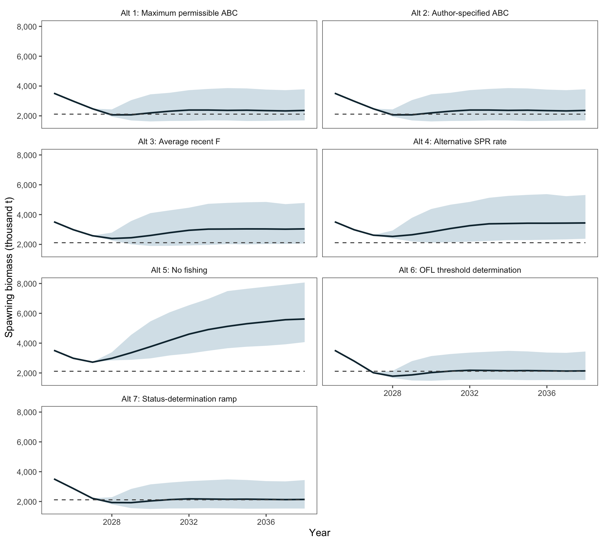
Projected spawning biomass remains above \(B_{35\%}\) under the harvest alternatives over the displayed horizon, with trajectories diverging after the fixed-catch years. Lines show simulation medians and ribbons show central 90% intervals (Figure 11).
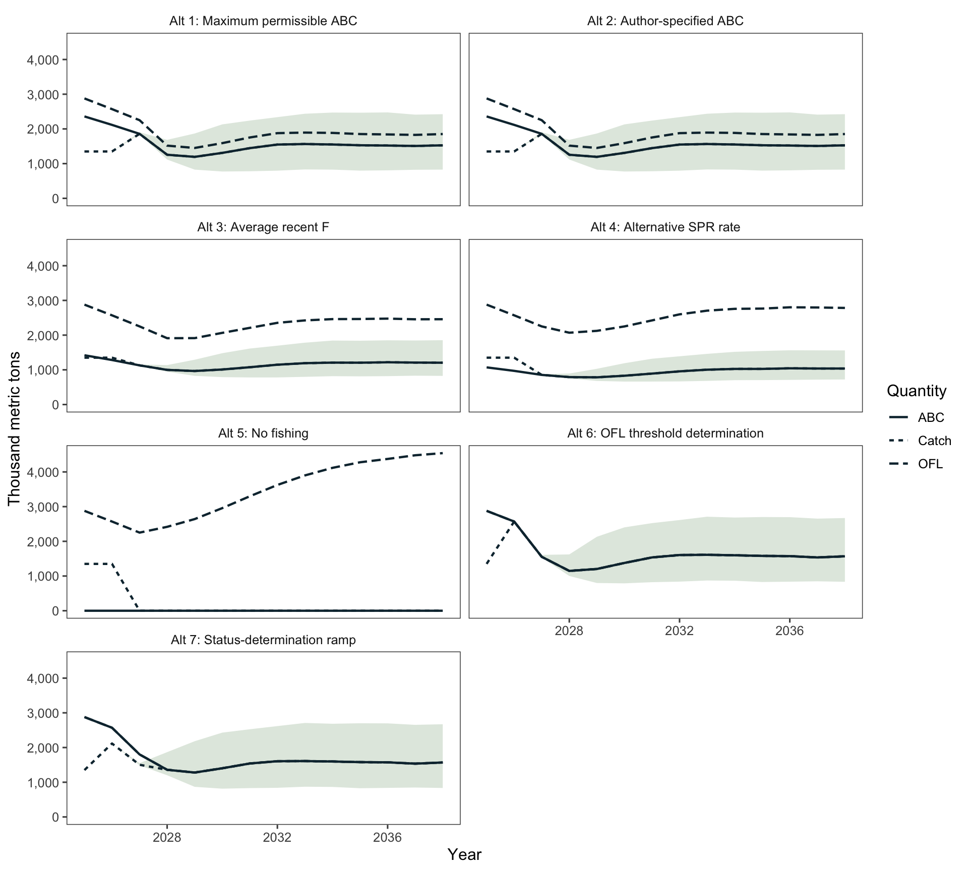
Projected catch, ABC, and OFL are identical during the fixed-catch period and then separate according to the alternative harvest rules (Figure 12).
7 Exploratory DSEM Recruitment Pathways
This section is the indicator-analysis pilot within a draft EBS pollock Ecosystem and Socioeconomic Profile (ESP), rather than an attempt to estimate the full pollock early-survival system. The BSAI Groundfish Plan Team recommended in 2021 that an EBS walleye pollock ESP be added to the list of future ESPs (Bering Sea/Aleutian Islands Groundfish Plan Team 2021). The analysis follows the sequence recommended in the AFSC causal-modeling guidance: define the outcome, build a literature-based mechanism table and generic DAG, select a small set of scientifically defensible graphs, retain a no-edge baseline, and compare all graphs on the same data (Monnahan and Shotwell 2026). The mechanism table and DAG draw on the January 2025 pollock workshop, the age-0 pollock working-group material, and the Tiger Team data-availability synthesis (Monnahan et al. 2026; Siddon et al. 2026; Alaska Fisheries Science Center Age-0 Pollock Causal-Modeling Working Group 2026; EBS Pollock Tiger Team 2026) and the EBS pollock Early Survival Pathways synthesis (J. N. Ianelli 2026).
The response is the Rceattle age-1 recruitment state. The two examples test late-summer SST in the cohort’s age-0 year and cold-pool extent in the following age-1 calendar year. They were selected because both have relatively long annual records and represent distinct, prespecified hypotheses. The analysis does not treat them as direct measurements of prey quality, energetic condition, cannibalism, or survival.
7.1 ESP development scope
The September product documents the justification, synthesis, generic DAG, mechanism table, and two illustrative fits. It does not substitute a long list of available covariates for a small set of causal hypotheses. The intended progression identifies the completed September analyses and the work deferred to November (Table 14). The full draft ESP structure is provided in Appendix A-3.
| Component | September draft | November target |
|---|---|---|
| Justification and outcome | Document the Plan Team request and define age-1 recruitment as the focal population response. | Confirm the focal response and management use with the ESP team. |
| Indicator synthesis | Provide a life-history synthesis, generic DAG, mechanism table, and data-availability review. | Update indicators through the ESP and Ecosystem Status Report data-collection process. |
| Candidate hypotheses | Retain two transparent proxy examples: age-0 late-summer SST and cold-pool extent. | Fit two to five defensible candidate DAGs that represent proximal mediators where data permit. |
| Indicator analysis | Compare the two single-edge examples and their combined diagnostic with the no-edge IID reference. | Add predictive, retrospective, timing, and observation-error checks to the candidate-DAG comparison. |
| Management use | Use results to illustrate the integrated Rceattle-DSEM workflow and identify data gaps. | Determine whether validated indicators are suitable for operational recruitment modeling or risk-table context. |
7.2 Mechanism table and generic DAG
The reduced mechanism table distinguishes processes that can be tested with the current annual data from biologically important mediators that remain intermittent or unavailable (Table 15). Expected signs describe the direction from the listed driver toward age-1 recruitment, whether directly or through the stated mechanism.
| Driver | Mechanism | Expected sign | Current coverage | Role here |
|---|---|---|---|---|
| Sea ice | Winter ice affects summer cold-pool extent, bloom conditions, and prey production. | Indirect | Annual physical index available; not fitted here | Upstream context |
| Cold-pool extent | A larger cold pool can separate juveniles from adult pollock and reduce cannibalism. | Positive | 42 annual values | Illustrative proxy edge |
| Age-0 late-summer SST | Warmer water can increase metabolic demand and reduce energy stored before winter. | Negative | 41 annual values | Illustrative proxy edge |
| Large copepods and euphausiids | Lipid-rich prey supports age-0 growth, energy storage, and overwinter survival. | Positive | Intermittent; 15 values in the current ESP cohort table | Unfitted mediator |
| Fall age-0 energy | Higher energy density and total energy increase overwinter survival to age 1. | Positive | Absent from the current annual cohort table | Priority mediator |
| Adult-pollock overlap | Greater adult-juvenile overlap increases cannibalism exposure. | Negative | A separate range-overlap product exists, but its survey timing is contemporaneous with the age-1 state | Deferred from the main example |
The generic DAG is adapted from the age-0 pollock working-group graph and retains both bottom-up and top-down routes (Figure 13). It makes the unobserved or intermittent mediators visible instead of allowing the two available physical proxies to stand in for entire mechanisms. Solid arrows are conceptual. Dashed arrows are the only recruitment paths fitted in this proof of concept.
flowchart LR
  ICE["Winter<br/>sea ice"] --> COLD["Summer<br/>cold pool"]
  ICE --> BLOOM["Bloom timing<br/>and production"]
  ICE --> SST["Age-0 late-<br/>summer SST"]

  BLOOM --> PREY["Large copepods<br/>and euphausiids"]
  SST --> PREY
  PREY --> A0["Age-0 abundance,<br/>growth, and size"]
  PREY --> ENERGY["Age-0 diet lipid,<br/>energy density,<br/>and total energy"]
  A0 --> ENERGY
  ENERGY --> WINTER["Overwinter<br/>survival"]

  COLD --> SEP["Juvenile-adult<br/>spatial separation"]
  A0 --> JLOC["Juvenile<br/>distribution"]
  JLOC --> OVER["Cannibalism<br/>exposure"]
  SEP --> OVER
  ADULT["Adult pollock<br/>biomass and distribution"] --> OVER
  OVER --> PSURV["Predation<br/>survival"]

  WINTER --> REC["Age-1<br/>recruitment"]
  PSURV --> REC

  SST -. "fitted proxy edge" .-> REC
  COLD -. "fitted proxy edge" .-> REC

  classDef physical fill:#e8f2f7,stroke:#26739b,stroke-width:2px,color:#1f2933;
  classDef prey fill:#ecf5eb,stroke:#6b8f24,stroke-width:2px,color:#1f2933;
  classDef juvenile fill:#fff3df,stroke:#c68519,stroke-width:2px,color:#1f2933;
  classDef predator fill:#fdf2e8,stroke:#c8523f,stroke-width:2px,color:#1f2933;
  classDef survival fill:#e8f6f2,stroke:#13856f,stroke-width:2px,color:#1f2933;
  class ICE,COLD,SST physical;
  class BLOOM,PREY prey;
  class A0,ENERGY,JLOC juvenile;
  class SEP,ADULT,OVER predator;
  class WINTER,PSURV,REC survival;
The generic graph is intentionally broader than the statistical examples. It shows that a negative SST coefficient would be consistent with an energetic constraint, but would not identify prey quality, age-0 energy, or overwinter survival as the active mediator. Likewise, a cold-pool coefficient would be a proxy for spatial separation and cannibalism unless overlap and mortality were observed directly.
7.3 Two illustrative hypotheses
The proof of concept compares two single-edge hypotheses with a common reference:
- Energetic-condition proxy: higher age-0 late-summer SST is associated with lower age-1 recruitment because warmer conditions can increase metabolic demand and reduce fall energy reserves (Heintz et al. 2013; Siddon et al. 2013; Duffy-Anderson et al. 2016).
- Spatial-separation proxy: larger cold-pool extent is associated with higher age-1 recruitment because it can reduce juvenile-adult spatial overlap and cannibalism.
The age-0 SST value is carried forward to the DSEM row for that cohort’s age-1 recruitment. The zero-lag path is therefore cohort-aligned rather than a claim that SST was measured in the age-1 year. In this section “IID” refers to the no-recruitment-edge reference model. The combined model is retained as a limited diagnostic of whether the two proxy edges add information when fitted together; it is not a third mechanistic hypothesis.
All four specifications use the same observation-year universe, missingness pattern, standardization, and AR(1) processes for the observed covariates. Within this common data block, AIC compares relative fit after accounting for model complexity. The percentage reduction in residual recruitment variation compares each model’s estimated unexplained recruitment variance with the IID reference. It is an in-sample description, not a causal R-squared or a predictive-skill score.
7.4 Illustrative results
| Model | AIC | Delta AIC | Residual variation reduced (%) |
|---|---|---|---|
| Age-0 late-summer SST | 4,144.56 | 0.00 | 10.5 |
| Cold pool + age-0 late-summer SST | 4,146.19 | 1.63 | 12.0 |
| IID recruitment deviations | 4,146.81 | 2.25 | 0.0 |
| Cold pool | 4,148.66 | 4.11 | 0.3 |
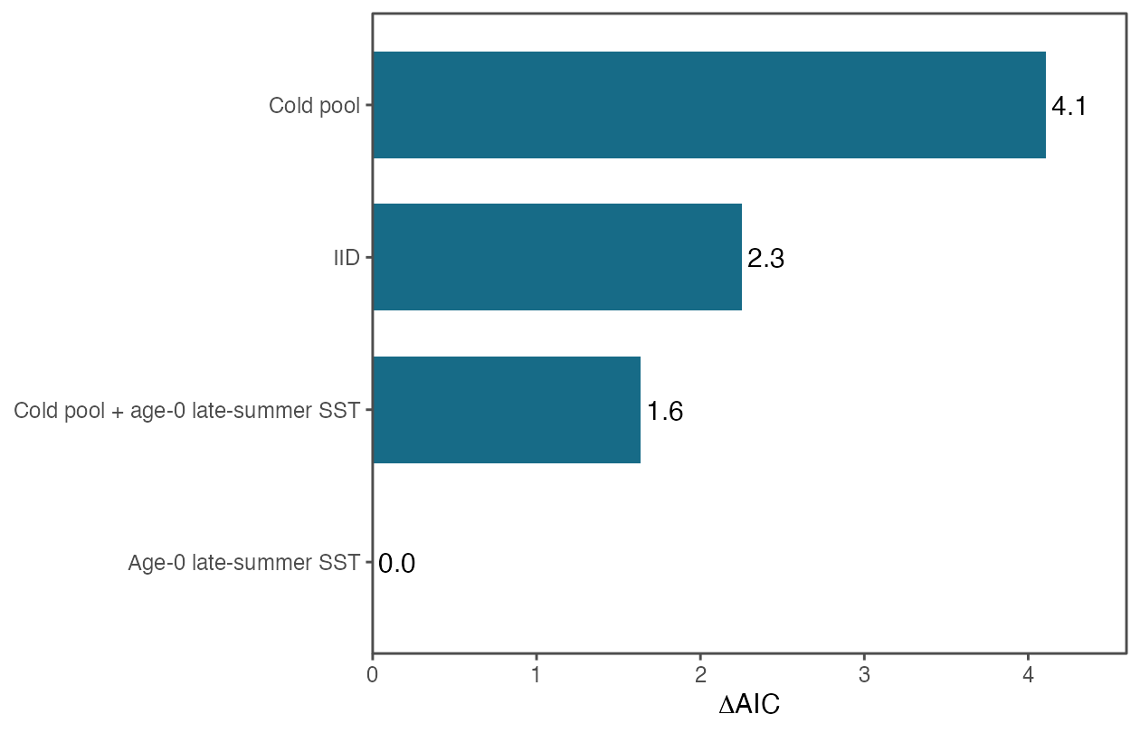
All four fits fully met the convergence criteria, had positive-definite Hessians, and had maximum absolute gradients no larger than 9.4e-05. The age-0 late-summer SST model had the lowest AIC and reduced estimated residual recruitment variation by 10.5% relative to IID. The cold-pool-only model reduced residual variation by 0.3% and had higher AIC than IID. The combined model reduced residual variation by 12.0%, but its additional parameter left its AIC above the SST-only model (Table 16; Figure 14).
| Covariate | Estimate | Standard error | Lower 95% | Upper 95% |
|---|---|---|---|---|
| Cold pool | ||||
| Cold pool | 0.041 | 0.107 | −0.169 | 0.251 |
| Age-0 late-summer SST | ||||
| Age-0 late-summer SST | −0.222 | 0.104 | −0.426 | −0.017 |
| Cold pool + age-0 late-summer SST | ||||
| Cold pool | −0.069 | 0.114 | −0.292 | 0.153 |
| Age-0 late-summer SST | −0.254 | 0.118 | −0.485 | −0.024 |
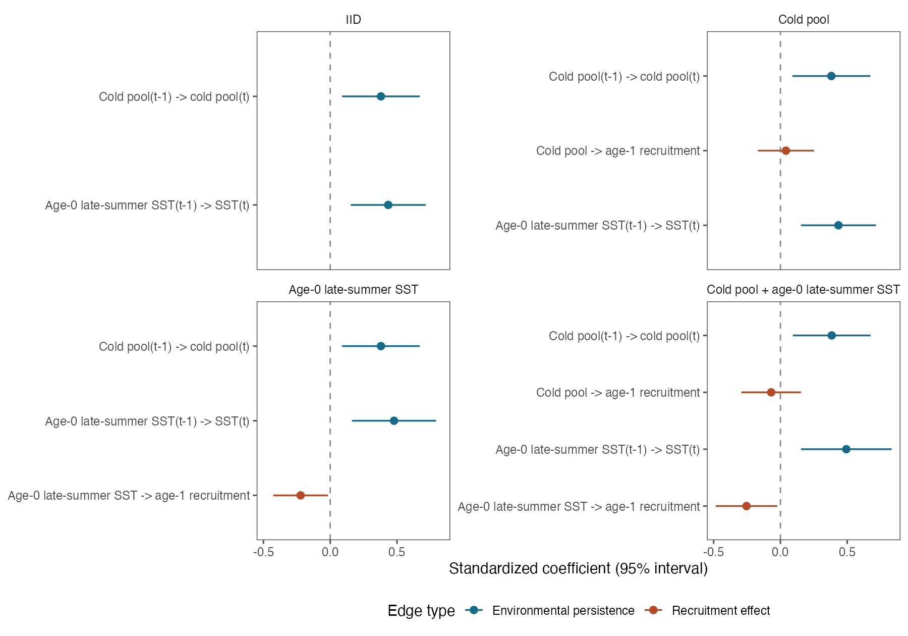
The SST coefficient was negative and its interval excluded zero in both the single-edge and combined models. The cold-pool coefficient was small and its interval included zero in both models. In plain language, the current annual data contain a modest in-sample association consistent with the warm-year energetic-constraint hypothesis, while the direct cold-pool proxy edge received little support. Neither result establishes the intervening mechanism (Table 17; Figure 15).
The missingness-preserving randomization check replaced both environmental series with independent standard-normal values using seed 20260812. None of the randomized recruitment paths improved on the randomized IID model: their delta AIC values ranged from 1.03 to 2.95, and every randomized path interval included zero. This is a basic check against an identical signal arising from arbitrary series with the same gaps; it does not replace out-of-sample validation.
7.5 Interpretation and next test
This proof of concept supports keeping the candidate set small. The SST result is useful as an illustration of the Rceattle-DSEM connection, but SST is an upstream proxy. The next scientifically stronger test is to insert a proximal mediator from the mechanism table: fall age-0 total energy or energy density, followed by a lipid-rich large-copepod/euphausiid index when enough cohort years are available (Eisner et al. 2020; Heintz et al. 2013; Siddon et al. 2013). That sequence would test whether the SST association weakens when the hypothesized energetic path is represented directly.
A top-down overlap example should return only after its timing and uncertainty are aligned with the age-0-to-age-1 survival interval. The available adult-pollock overlap product is informative, but its survey occurs after the start-of-year age-1 state and it is partly population-derived. Including it here would blur a causal example with a contemporaneous association.
Before either proxy is considered for operational recruitment inference, the paths should be tested with terminal-year or blocked prediction, retrospective stability, alternative cohort timing, and observation-error sensitivity. These DSEM results remain separate from the assessment configuration and projection results.
8 Summary and conclusions
When Rceattle parameters and fishery selectivity are set to the values used in the ADMB model, Rceattle reproduces spawning biomass and predicted catch to numerical precision. This establishes agreement in the tested population-dynamics calculations and parameter mapping. When Rceattle is fit to the data, the trajectories differ more, and the residual least-identified direction remains in the shared ATS/AVO annual selectivity deviations. The added ATS/AVO coefficient-increment penalty reduced the condition number below the convergence-warning threshold.
The diagnostic results identify a focused development path for the September 2026 Plan Team evaluation. The Rceattle fit fully met the convergence criteria. Composition OSA residuals remain underdispersed. Nine terminal-year-consistent peels converge successfully and produce positive retrospective bias in spawning biomass, total biomass, and recruitment, together with negative bias in fishing mortality. The historical 2D AR1 sensitivity did not converge and retains its research status. The 50-jitter diagnostic recovered the best solution 48 times and found a poorer mode twice.
The scaled-back DSEM proof of concept compared two prespecified proxy edges with the no-edge IID reference. The age-0 late-summer SST model had the lowest AIC and reduced estimated residual recruitment variation by 10.5% relative to IID. The cold-pool edge received little support. This result illustrates the Rceattle-DSEM connection, but the annual data do not yet represent the prey, age-0 energy, overwinter-survival, and cannibalism mediators required to attribute the association to a causal mechanism.
Immediate work should retain the ADMB-to-Rceattle comparison as a repeatable numerical check, evaluate selectivity and survey influence on the retrospective pattern, and continue sensitivity checks for the shared ATS/AVO annual selectivity deviations. Given acceptance in other applications and the proven bridging aspects, we feel this approach should be adopted for operational management advice for November/December 2026. Future refinements will explore trade-offs in fitting data in alternative ways (e.g., using random effects approaches for selectivity variability, selecting alternatives to the robust-multinomial approach used in this example). The exploratory DSEM work provides a reproducible approach for adding cohort-aligned covariates, while remaining separate from the final assessment configuration and projection results.
Rceattle is broadly used beyond this EBS pollock application. The framework has been applied to single- and multispecies groundfish cases in the eastern Bering Sea and Gulf of Alaska, including configurations for pollock, Pacific cod, and arrowtooth flounder. Its shared data structure accommodates one or more stocks, one- or two-sex population dynamics, and multiple fisheries and surveys. The present bridge therefore represents an application of a broader assessment framework rather than a model developed only for EBS pollock.
Rceattle is also under active development. Continued work on its TMB model, data interfaces, diagnostics, simulation tools, and documentation is expanding the set of configurations that can be represented and tested. This development is an advantage for future assessment work, but it also reinforces the need to record package versions, preserve model inputs and fitted outputs, and repeat the ADMB bridge and convergence checks when consequential components change.
Only part of the available Rceattle feature set was explored here. This study focused on a single-species age-structured configuration, ADMB parameter mapping, selectivity, composition fitting, standard diagnostics, projections, and an exploratory DSEM extension. It did not fully evaluate joint multispecies estimation, bioenergetics-based predation mortality, estimable growth, environmental linkages across other biological parameters, alternative harvest control rules and climate scenarios, or closed-loop management strategy evaluation. These capabilities provide a substantial agenda for future testing, but each should be evaluated through controlled sensitivities and diagnostics before contributing to operational EBS pollock advice.
References
Alaska Fisheries Science Center Age-0 Pollock Causal-Modeling Working Group. 2026. Age-0 Pollock DAG. Google Slides working document. https://docs.google.com/presentation/d/1tninaCS9iSGh9alXp7jGIcr1cE0owcrlE8yepBW2oYw/.
Alaska Fisheries Science Center Ecosystem and Socioeconomic Profile Coordination Team. 2026. Blank ESP Tables and Figures. Unpublished national ESP template.
Bering Sea/Aleutian Islands Groundfish Plan Team. 2021. Minutes of the Bering Sea/Aleutian Islands Groundfish Plan Team, September 22–23, 2021. North Pacific Fishery Management Council meeting minutes. https://meetings.npfmc.org/CommentReview/DownloadFile?p=f0e75d8e-4fbb-474a-a4aa-4c091cbc637b.pdf\&fileName=C6\%20September\%202021\%20BSAI\%20GPT\%20Minutes.pdf.
Duffy-Anderson, Janet T., Steven J. Barbeaux, Edward V. Farley, et al. 2016. “The Critical First Year of Life of Walleye Pollock (Gadus chalcogrammus) in the Eastern Bering Sea: Implications for Recruitment and Future Research.” Deep-Sea Research Part II: Topical Studies in Oceanography 134: 283–301. https://doi.org/10.1016/j.dsr2.2015.02.001.
EBS Pollock Tiger Team. 2026. EBS Pollock: Eco Framework. Tiger Team Google Slides working document. https://docs.google.com/presentation/d/1bSajTmPfWmiXqK6sHMOT8DZevklJ8ZzRrJEN2QdtIfw/.
Eisner, Lisa B., Ellen M. Yasumiishi, Alexander G. Andrews, and Cecilia A. O’Leary. 2020. “Large Copepods as Leading Indicators of Walleye Pollock Recruitment in the Southeastern Bering Sea: Sample-Based and Spatio-Temporal Model (VAST) Results.” Fisheries Research 232: 105720. https://doi.org/10.1016/j.fishres.2020.105720.
Heintz, Ron A., Elizabeth C. Siddon, Edward V. Farley, and Jeffrey M. Napp. 2013. “Correlation Between Recruitment and Fall Condition of Age-0 Pollock (Theragra chalcogramma) from the Eastern Bering Sea Under Varying Climate Conditions.” Deep-Sea Research Part II: Topical Studies in Oceanography 94: 150–56. https://doi.org/10.1016/j.dsr2.2013.04.006.
Ianelli, James N. 2026. Eastern Bering Sea Walleye Pollock Early Survival Pathways. Quarto website. https://afsc-assessments.github.io/ebswp_esp/.
Ianelli, Jim. 2026. spmR: Standard Projection Model. http://afsc-assessments.github.io/spmR/.
Monnahan, Cole C., David McGowan, James N. Ianelli, Bridgett Ferriss, and Lauren A. Rogers, eds. 2026. Proceedings of the Workshop on Walleye Pollock Biology and Ecology. Draft Alaska Fisheries Science Center processed report.
Monnahan, Cole C., and S. Kalei Shotwell. 2026. Tentative Good Practices for AFSC Causal Modeling. Living Alaska Fisheries Science Center working document. https://docs.google.com/document/d/1ZyAQ-WtdqErHFxT567qQunvJI8WF-bi6ygqpzkPHvUI/.
Schiano, Samantha, Sophie Breitbart, and Steve Saul. 2026. Asar: Build NOAA Stock Assessment Report. https://github.com/nmfs-ost/asar.
Shotwell, S. Kalei, Jenny Bigman, and Russel Dame, eds. 2026. Ecosystem and Socioeconomic Profile of the Arrowtooth Flounder Stock in the Gulf of Alaska. Appendix 7A in the Gulf of Alaska arrowtooth flounder stock assessment.
Siddon, Elizabeth C., Ron A. Heintz, and Franz J. Mueter. 2013. “Conceptual Model of Energy Allocation in Walleye Pollock (Theragra chalcogramma) from Age-0 to Age-1 in the Southeastern Bering Sea.” Deep-Sea Research Part II: Topical Studies in Oceanography 94: 140–49. https://doi.org/10.1016/j.dsr2.2012.12.007.
Siddon, Elizabeth C., S. Kalei Shotwell, and James N. Ianelli. 2026. Age-0 Pollock DSEM Noteworthy: Eastern Bering Sea Walleye Pollock Early Survival Pathways. Unpublished Alaska Fisheries Science Center working document.
Vehtari, Aki, Andrew Gelman, and Jonah Gabry. 2017. “Practical Bayesian Model Evaluation Using Leave-One-Out Cross-Validation and WAIC.” Statistics and Computing 27 (5): 1413–32. https://doi.org/10.1007/s11222-016-9696-4.
Vehtari, Aki, Daniel Simpson, Andrew Gelman, Yuling Yao, and Jonah Gabry. 2024. “Pareto Smoothed Importance Sampling.” Journal of Machine Learning Research 25 (72): 1–58. https://jmlr.org/papers/v25/19-556.html.
Appendices
A-1 Reproducibility and analysis sequence
The working paper is rendered from saved model and diagnostic products so that building the document does not repeat long model fits. The commands below are run from the project directory, in the order shown when an earlier product is required by a later analysis.
- The input-preparation script documents the transformations used to prepare the aligned Rceattle workbook; its precursor workbook is regenerated with
Rscript "2024 EBS pollock setup data.R". The frozen workbook used for the reported fit isData/EBS_24_pollock_m23_rceattle_full_1964-2024.xlsx. The same script documents the modified ADMB reference rebuild, run ascd ADMB/m23_rceattle_full && admb pm && ./pm -nox -iprint 150after the ADMB executable directory has been added toPATH. - The two-stage fitting script fits the reported Rceattle configuration and the 2D age-by-year AR1 sensitivity with
Rscript "2024 EBS pollock.R". The 5.8.1 summary script then generates the fitted-model summaries and standard-multinomial sensitivity usingRscript R/finalize_rceattle_5_8_1_analysis.R. - The ADMB bridge runner sets the Rceattle parameters and realized selectivity to the ADMB values and saves the trajectory, likelihood, and gradient comparisons with
Rscript R/run_canonical_pm_forward_bridge.R. - The OSA runner generates the saved OSA residuals with
Rscript R/run_canonical_pm_diagnostics.R. The retrospective script runs the nine terminal-year-consistent peels withRscript "2024 EBS pollock two-stage retrospectives.R". - The 5.8.1 self-test runner generates 50 phased simulations with
Rscript R/run_rceattle_5_8_1_self_test.R. The restart runner repeats the same simulations from the estimated solution withRscript R/run_rceattle_5_8_1_self_test_restart.R, and the validation summarizer is run withRscript R/summarize_rceattle_5_8_1_validation.R. - The projection runner, which uses the Rceattle-to-SPM input writer, generates the seven-scenario and fixed-catch projection products with
Rscript R/run_spmr_tier3_projection.R. - The DSEM script runs the four observed-covariate models with
Rscript "2024 EBS pollock DSEM proof of concept.R"and the missingness-preserving randomized controls withRscript "2024 EBS pollock DSEM proof of concept.R" --randomized. - After these saved products are available, the report-input preparation script extracts the compact quantities, diagnostics, and trajectories needed by the document with
Rscript R/prepare_report_inputs.R. The HTML and PDF are then generated together withscripts/render_report.sh.
The report inventory identifies the model inputs, saved diagnostic products, scripts, and projection outputs needed to reproduce the working paper (Table 18).
| Role | Location | Available | Size |
|---|---|---|---|
| Prepared model-input workbook | Local workbook | TRUE | 135.1 KB |
| BTS covariance input | Local data file | TRUE | 12.7 KB |
| Compact report-ready Rceattle products | Versioned R serialized-data (RDS) file | TRUE | 131.5 KB |
| OSA residuals | Local RDS file | TRUE | 91.2 KB |
| OSA diagnostics | Local RDS file | TRUE | 1.1 KB |
| Compact nine-peel retrospective products | Versioned RDS file | TRUE | 21.1 KB |
| Nine-peel Mohn's rho summary | Local CSV file | TRUE | 0.2 KB |
| Nine-peel retrospective script | Local R script | TRUE | 9.7 KB |
| ADMB-to-Rceattle comparison output | Local RDS file | TRUE | 650.8 KB |
| Rceattle 5.8.1 self-test summary | Local CSV file | TRUE | 0.5 KB |
| Rceattle 5.8.1 truncation diagnostics | Local CSV file | TRUE | 0.4 KB |
| Rceattle 5.8.1 restart comparison | Local CSV file | TRUE | 3.8 KB |
| Rceattle 5.8.1 jitter summary | Local CSV file | TRUE | 2.3 KB |
| ADMB-to-Rceattle comparison summary | Local comma-separated-values (CSV) file | TRUE | 1.0 KB |
| Rceattle fitting script | Local R script | TRUE | 15.7 KB |
| Diagnostics script | Local R script | TRUE | 4.9 KB |
| Next-assessment update script | Local R script | TRUE | 2.6 KB |
| ADMB comparison script | Local R script | TRUE | 10.1 KB |
| Rceattle-to-SPM input writer | Local R script | TRUE | 8.7 KB |
| spmR Tier 3 projection runner | Local R script | TRUE | 1.5 KB |
| SPM projection manifest | Local CSV file | TRUE | 0.5 KB |
| Exploratory DSEM script | Local R script | TRUE | 17.1 KB |
| DSEM model comparison | Local CSV file | TRUE | 0.5 KB |
| DSEM recruitment-path estimates | Local CSV file | TRUE | 3.1 KB |
| Randomized DSEM control | Local CSV file | TRUE | 0.5 KB |
| DSEM AIC comparison figure | Local PNG file | TRUE | 24.3 KB |
| DSEM edge-coefficient figure | Local PNG file | TRUE | 100.9 KB |
| Compact report-input manifest | Versioned CSV file | TRUE | 6.9 KB |
R version 4.6.1 (2026-06-24)
Platform: aarch64-apple-darwin23
Running under: macOS Tahoe 26.6.2

Matrix products: default
BLAS:   /Library/Frameworks/R.framework/Versions/4.6/Resources/lib/libRblas.0.dylib
LAPACK: /Library/Frameworks/R.framework/Versions/4.6/Resources/lib/libRlapack.dylib;  LAPACK version 3.12.1

locale:
[1] C.UTF-8/C.UTF-8/C.UTF-8/C/C.UTF-8/C.UTF-8

time zone: Europe/Brussels
tzcode source: internal

attached base packages:
[1] stats     graphics  grDevices utils     datasets  methods   base

other attached packages:
 [1] tidyr_1.3.2     tibble_3.3.1    scales_1.4.0    readr_2.2.0
 [5] knitr_1.51      gt_1.3.0        ggthemes_5.2.0  ggplot2_4.0.3
 [9] ggridges_0.5.7  dplyr_1.2.1     asar_2.5.0.9000 afscOSA_0.0.1

loaded via namespace only:
 [1] sass_0.4.10        generics_0.1.4     xml2_1.6.0         lattice_0.22-9
 [5] stringi_1.8.7      hms_1.1.4          digest_0.6.39      magrittr_2.0.5
 [9] evaluate_1.0.5     grid_4.6.1         RColorBrewer_1.1-3 fastmap_1.2.0
[13] plyr_1.8.9         jsonlite_2.0.0     Matrix_1.7-5       purrr_1.2.2
[17] viridisLite_0.4.3  cli_3.6.6          rlang_1.3.0        crayon_1.5.3
[21] litedown_0.9       commonmark_2.0.0   cowplot_1.2.0      bit64_4.8.2
[25] base64enc_0.1-6    withr_3.0.3        yaml_2.3.12        otel_0.2.0
[29] tools_4.6.1        parallel_4.6.1     reshape2_1.4.5     tzdb_0.5.0
[33] png_0.1-9          vctrs_0.7.3        R6_2.6.1           lifecycle_1.0.5
[37] stringr_1.6.0      fs_2.1.0           htmlwidgets_1.6.4  bit_4.6.0
[41] vroom_1.7.1        pkgconfig_2.0.3    pillar_1.11.1      gtable_0.3.6
[45] Rcpp_1.1.2         glue_1.8.1         xfun_0.60          tidyselect_1.2.1
[49] farver_2.1.2       htmltools_0.5.9    labeling_0.4.3     rmarkdown_2.31
[53] TMB_1.9.21         compiler_4.6.1     S7_0.2.2           markdown_2.0
A-2 Rceattle-to-spmR projection bridge
The projection bridge is a deterministic file adapter rather than a second assessment fit. The input writer reads the saved nonparametric_pm Rceattle object, extracts the population state, biological schedules, fishery schedule, and historical series needed by the Standard Projection Model (SPM), and writes them in the SPM pm.prj format. It also writes the projection controls in spm.dat. The projection runner passes those files to spmR::runSPM(..., engine = "admb"), which executes the validated SPM binary and returns the simulation-level output used by the report.
The adapter preserves the terminal assessment state and makes each conversion explicit. Numbers at age, natural mortality, and the weight schedules are passed on their Rceattle scales. With abundance in millions of fish and weight in kilograms, their product has units of thousand metric tons. Maturity is divided by its maximum, matching the SPM input convention used for this stock. The spawning-month encodings differ by one because Rceattle records elapsed months and SPM uses a one-based calendar month; both represent survival through 0.25 of the year (Table 19).
| SPM field | Rceattle source | Transformation and years |
|---|---|---|
| Average recent F | quantities: F_spp | Arithmetic mean for 2020--2024; used by Alternative 3 |
| Natural mortality at age | quantities: M_at_age | Terminal-year schedule (2024) |
| Maturity at age | data_list: maturity | Divided by its maximum to match the SPM convention |
| Spawning weight at age | data_list: weight and ssb_wt_index | Terminal-year spawning-weight schedule |
| Fishery weight at age | data_list: weight, fishery index | Terminal-year fishery-weight schedule |
| Fishery selectivity at age | quantities: sel_at_age for Fishery | Arithmetic mean at each age for 2020--2024 |
| Terminal numbers at age | quantities: N_at_age | Terminal assessment state (2024) |
| Recruitment history | quantities: R | Annual age-1 recruitment for 1978--2024 |
| Spawning-biomass history | quantities: ssb | Annual spawning biomass for 1977--2023 |
| Spawning month | data_list: spawn_month = 3 | Written as SPM Spawnmo = 4; both equal 0.25 year |
Annual Rceattle fishery selectivity is already normalized to a mean of one across ages. The projection schedule is calculated as the arithmetic mean at each age across 2020–2024; averaging these normalized annual curves retains a mean of one. This five-year schedule replaces the former terminal-year-only curve. The writer saves the five contributing curves in fishery_selectivity_recent_years.csv, the applied average in age_schedules.csv, and the rule and exact years in lineage.csv. Thus the projection input can be reconstructed without reading values back from the formatted pm.prj file.
The spm.dat file starts projections in 2025, runs 14 projection years and 1,000 simulations, and requests all seven Tier 3 alternatives. Catch is fixed at 1,350 thousand t in 2025 and 2026 before the alternatives diverge. A separate call uses Alternative 2 with catch fixed at 1,300 thousand t for 2025–2032. The writer copies the validated SPM executable and tacpar.dat control file into each run directory. manifest.csv records the role and presence of every required input, while lineage.csv records the terminal year, software versions, selectivity rule, and averaging years.
The saved products passed all file and field consistency checks. These checks do not replace review of the harvest assumptions or the biological appropriateness of a five-year selectivity average (Table 20).
The means formerly displayed in the long main-text table remain available as a downloadable CSV. This file retains every alternative and projection year in a compact, machine-readable form. The underlying simulation-level output remains in the saved analysis products but is omitted from the report because of its size.
| Check | Result | Evidence |
|---|---|---|
| Required projection files | Pass | 6 of 6 manifest targets present |
| Recent selectivity years | Pass | 2020, 2021, 2022, 2023, 2024 |
| Applied five-year selectivity mean | Pass | maximum absolute difference = 3.996803e-15 |
| Projection alternatives | Pass | 1, 2, 3, 4, 5, 6, 7 |
| Projection start year | Pass | 2025 |
A-3 Draft EBS pollock ESP development framework
The most effective way to integrate the ecosystem work into this working paper is to keep the concise DSEM pilot in Section 7 and develop the full ESP as an appendix. This preserves the assessment narrative while giving the ESP its own standard structure, evidence trail, and update cycle. The scaffold below adapts the national ESP tables and the 2026 Gulf of Alaska arrowtooth flounder ESP (Alaska Fisheries Science Center Ecosystem and Socioeconomic Profile Coordination Team 2026; Shotwell et al. 2026). It is a September draft: the indicator synthesis and proposed causal structure are present, while the final indicator updates, expanded candidate-DAG comparison, and management summary are November deliverables. The proposed components and their present status show which elements are complete and which remain scheduled for November (Table 21).
| ESP component | EBS pollock content | Current status |
|---|---|---|
| Executive summary | ABC/TAC relevance, predictive and contextual indicators, principal data gaps. | Write after the November indicator analysis. |
| Introduction and justification | 2021 BSAI Plan Team request; focal response is age-1 recruitment and its early-survival mechanisms. | Justification documented; team review pending. |
| Data | Assessment states, physical indices, plankton and prey indices, age-0 condition, predation/overlap products, and selected socioeconomic series. | Inventory started; several proximal biological series remain short or intermittent. |
| Indicator synthesis | Life-history table, conceptual diagram, generic DAG, and mechanism table developed from the workshop and working-group material. | Draft synthesis presented here and in Section 7. |
| Proposed indicators | A small set selected by mechanism, timing, record length, uncertainty, and availability rather than correlation alone. | SST and cold pool illustrate the workflow; age-0 energy and lipid-rich prey are priorities. |
| Indicator assessment | Current condition, trends, uncertainty, and interpretation for ecosystem and socioeconomic indicators. | Complete after current-year ESP and ESR data collection. |
| Indicator analysis | No-edge reference, candidate DAGs, common-data AIC, path estimates, residual-variance change, predictive checks, and scientific sign checks. | Two proxy examples completed; expanded candidate-DAG analysis deferred to November. |
| Data gaps and priorities | Fall age-0 energy, prey lipid/abundance, bloom-prey match timing, juvenile-adult overlap, and consistent observation-error information. | Priorities identified; feasible annual products require team confirmation. |
| Conclusion and management use | Separate predictive indicators from contextual indicators and state whether each is suitable for recruitment modeling, the risk table, or monitoring only. | Complete after validation and team review. |
The draft life-history synthesis condenses the standard ESP table to the stages and information needed for the recruitment question (Table 22). A later stand-alone ESP can expand each stage into the national-template fields for habitat and distribution, phenology, growth, energetics, diet, and predators or competitors.
| Stage | Process emphasized | Available evidence | Priority gap |
|---|---|---|---|
| Spawning and eggs | Adult condition, spawn timing and location, egg development, and transport. | Adult condition and physical indices are regularly available. | Cohort-specific egg production and transport exposure. |
| Larvae | Bloom timing, prey match, transport, temperature-dependent growth, and predation. | Physical forcing is available; biological observations are less consistent. | Annual bloom-prey match and larval survival indices. |
| Young of year | Prey quantity and lipid quality, growth, distribution, and accumulation of fall energy. | SST is long; prey and condition series are shorter or intermittent. | Consistent fall age-0 abundance, diet lipid, energy density, and total energy. |
| Overwinter age 0 to age 1 | Energy reserves, metabolic demand, winter severity, and predation determine survival. | Physical proxies and modeled recruitment are available. | Direct annual overwinter-survival observations and uncertainty. |
| Juvenile and pre-recruit | Spatial overlap with adults and other predators affects cannibalism and natural mortality. | Adult abundance is long; overlap and mortality products require timing review. | Cohort-aligned juvenile-adult overlap and predation mortality. |
| Adult | Spawner abundance, condition, distribution, and cannibalism affect production and juvenile survival. | Assessment abundance, maturity, distribution, and condition products are available. | Separate maternal and density-dependent pathways from shared assessment information. |
The generic DAG in Section 7 serves as the initial full conceptual graph. The fitted SST and cold-pool graphs are deliberately simplified descendants of that graph, not a search across every available series. For November, each candidate graph should be traceable to a row in the mechanism table and should use the same analysis data block as the IID no-recruitment-edge reference. The final ESP should then report the causal statement, lag, expected sign, data limitations, path estimate, uncertainty, change in unexplained recruitment variation, and predictive check for every retained recruitment edge.
Fishery performance and socioeconomic indicators can be transferred from the SAFE after the biological indicator set is stable. They should occupy the standard socioeconomic synthesis and monitoring subsections rather than be inserted as recruitment causes unless a separate, defensible causal hypothesis requires them. This division keeps the integrated Rceattle-DSEM analysis focused on the population response while allowing the ESP appendix to inform both biological risk and TAC considerations.
A-4 Model fitting details
The fishery selectivity likelihood has multiple modes, so the reported Rceattle configuration used data-based fishery-selectivity starting values and two fitting stages. The first stage disabled the annual selectivity deviations to establish the selectivity and abundance scale. The second stage restored the deviations and used the first-stage solution as its initial values. This sequence produced a small maximum gradient and fully met the convergence criteria. With the direct ATS/AVO coefficient-increment penalty, the Hessian condition number was approximately 489,000; its weakest direction remained in the shared ATS/AVO annual selectivity deviations (sel_coff_dev) rather than fishery/CPUE.
The complete fitting sequence, including the empirical starting values and the two estimation stages, is in the two-stage fitting script and is run with Rscript "2024 EBS pollock.R". The nine-peel implementation is in the retrospective script and is run with Rscript "2024 EBS pollock two-stage retrospectives.R".
The retrospective peels repeat this sequence after recalculating the data-based selectivity starting values for each terminal year. Because sel_coff_dev contains annual random-walk increments at age, each peel fixes the terminal-year fishery and mirrored catch-per-unit-effort increments at zero. This holds their terminal selectivity-at-age curves at the preceding-year curves. The completed development components distinguish the accepted comparison, diagnostic work, and unresolved research sensitivities (Table 23).
| Item | Development component | Review result | Interpretation |
|---|---|---|---|
| 1 | Prepared Rceattle model-input workbook | Used the delivered workbook directly. | Input files are available and reproducible from stored files. |
| 2 | Rceattle fit and 2D AR1 sensitivity | The Rceattle fit completed; 2D AR1 received a FAIL convergence status. | The NonParametricPM configuration is the relevant Rceattle comparison; 2D AR1 is diagnostic only. |
| 3 | Convergence and model diagnostics | Structured convergence checks, OSA diagnostics, nine retrospective peels, 50 self-tests, and 50 jitters are saved. | The ATS/AVO coefficient-increment penalty resolves the prior Hessian-conditioning warning; two inferior jitter solutions remain. |
| 4 | Next-assessment data update workflow | Update script review is complete; execution awaits complete new-year observations. | Useful as a template only after complete new-year observations are inserted. |
| 5 | ADMB-to-Rceattle comparison diagnostics | Setting Rceattle to the ADMB values reproduces ADMB to rounding-scale precision. | This is the strongest evidence that the ADMB comparison is correct. |
A-5 Jitter-tests
The extended-diagnostics runner generates the 50 jitter fits with Rscript R/run_rceattle_5_8_1_extended_diagnostics.R.
The 50 phased jitter runs test sensitivity to dispersed starting values. Forty-eight returned to the best objective within numerical precision. Two received WARN status and reached an inferior mode with an objective increase of approximately 609.5. This reproduces the pre-existing multimodality and shows why convergence of one run is not sufficient evidence that the global mode was found. Forty-eight runs returned to the best mode and two reached the inferior mode (Table 24).
| Status | Runs | Minimum delta objective | Maximum delta objective |
|---|---|---|---|
| Criteria fully met | 48 | 0.000 | 0.000 |
| WARN | 2 | 609.548 | 609.548 |
A-6 2D age-by-year AR1 selectivity sensitivity
The penalized-effects initialization and subsequent Laplace fit are in the two-stage fitting script and are run with Rscript "2024 EBS pollock.R". A separate fixed-scale follow-up can be run with Rscript "2024 EBS pollock 2D AR1 fixed sd test.R"; it is a development check and is not the sensitivity summarized below.
The 2D AR1 sensitivity applied an age-by-year field to the shared fishery and catch-per-unit-effort selectivity block over 1964–2024. The age-year deviations were first fit as penalized effects to initialize the field and then integrated as random effects with a Laplace approximation. The initialized Laplace fit failed the gradient, Hessian, and bound checks. The estimated correlation and scale parameters are retained only as diagnostics (Table 25).
| Quantity | Rceattle parameter | Penalized effects | Random-effects fit |
|---|---|---|---|
| Year AR1 correlation | Sel_curve_pen1 | 0.584 | 0.947 |
| Age AR1 correlation | Sel_curve_pen2 | 0.120 | 0.098 |
| Selectivity deviation scale | sel_dev_log_sd | 0.500 | 0.379 |
| Correlations are on the -1 to 1 scale; the deviation scale is a positive standard deviation. The fit failed convergence checks. | |||
The failed random-effects fit had a maximum marginal gradient of 19.7 on rec_pars, a non-invertible Hessian, 61 log_F parameters at their configured bounds, and FAIL convergence status. Its selectivity surfaces differ visibly from both the ADMB reference and accepted Rceattle configuration, but the failed fit precludes biological interpretation (Figure 16).
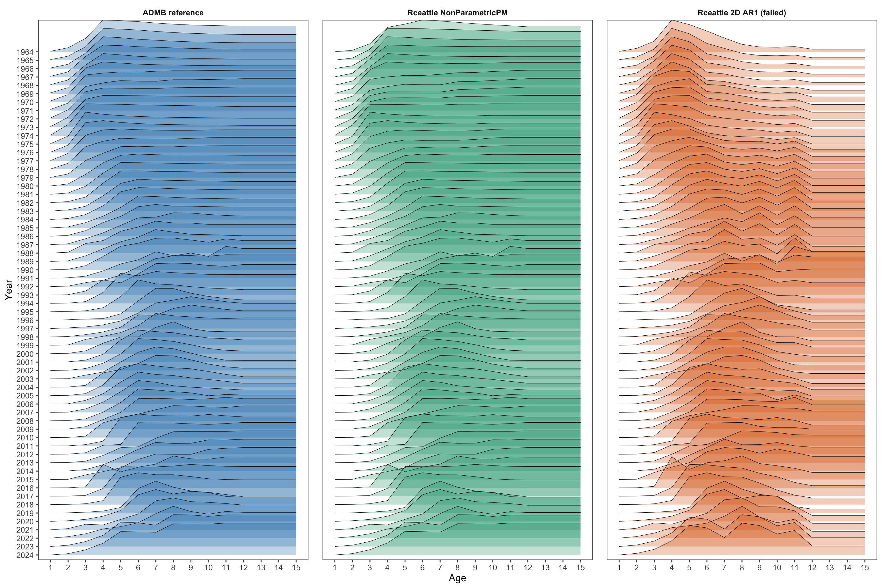
A-7 Observation continuity and case-deletion influence
This diagnostic separates whether an observation was available and used from how much the accepted fit changes when a fitted sampling event is removed. The observation-continuity panel (Figure 17) uses an explicit assessment-input schedule: annual for the fishery, BTS, and AVO rows and even years for ATS rows. Years after 2024 are shown only to distinguish the current fitted span; the schedule does not imply a commitment about future field operations.
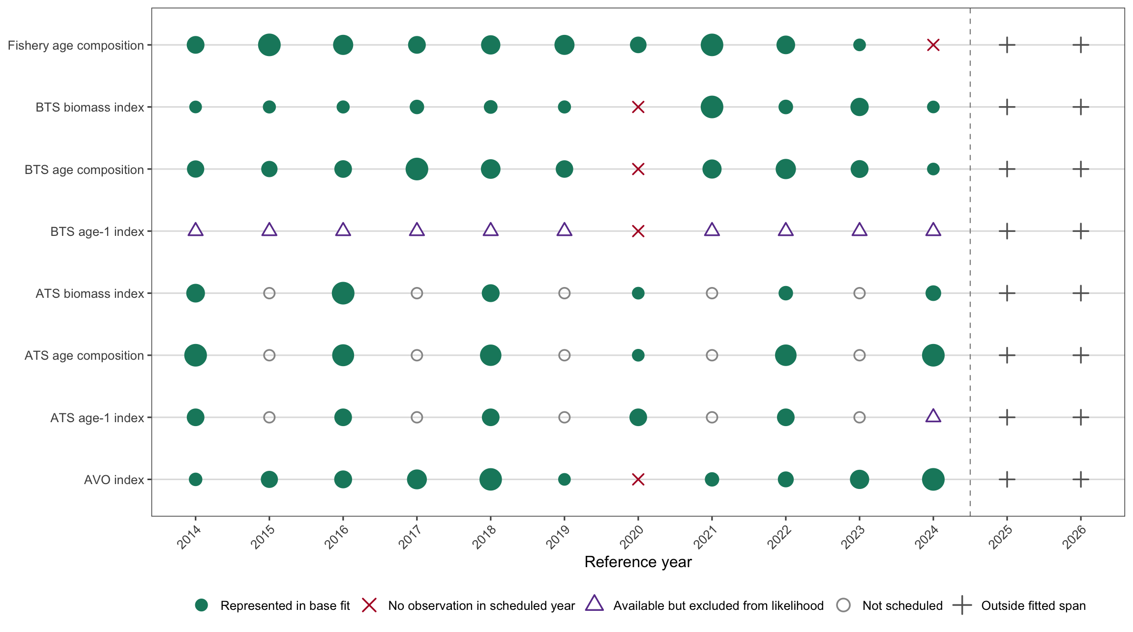
The standalone BTS age-1 series is present in the input workbook but its fleet control is Off; those observations are therefore not represented in the likelihood. The ATS age-1 index is active through 2022, whereas its 2024 row is negative-year coded and excluded. The fishery age-composition series ends in 2023, leaving a scheduled 2024 gap. The 2020 BTS and AVO gaps are also visible, while odd ATS years are correctly classified as not scheduled rather than missing.
Each composition deletion removed the complete fleet-year row, retaining its age bins as one multinomial sampling event. Each index deletion removed one fleet-year row. For the BTS biomass index this is an explicit case deletion from the joint covariance likelihood, not a claim that Cholesky-whitened OSA terms are independent annual likelihoods. The 12 controlled refits retained the accepted parameter map, model controls, robustifying constant (c = 0.001), and full-data solution as their starting point. The diagnostic runner writes a continuity inventory, refit manifest, summary, assessment-year trajectories, and objective-component totals. The terminal changes are displayed in Figure 18 and summarized in Table 26.
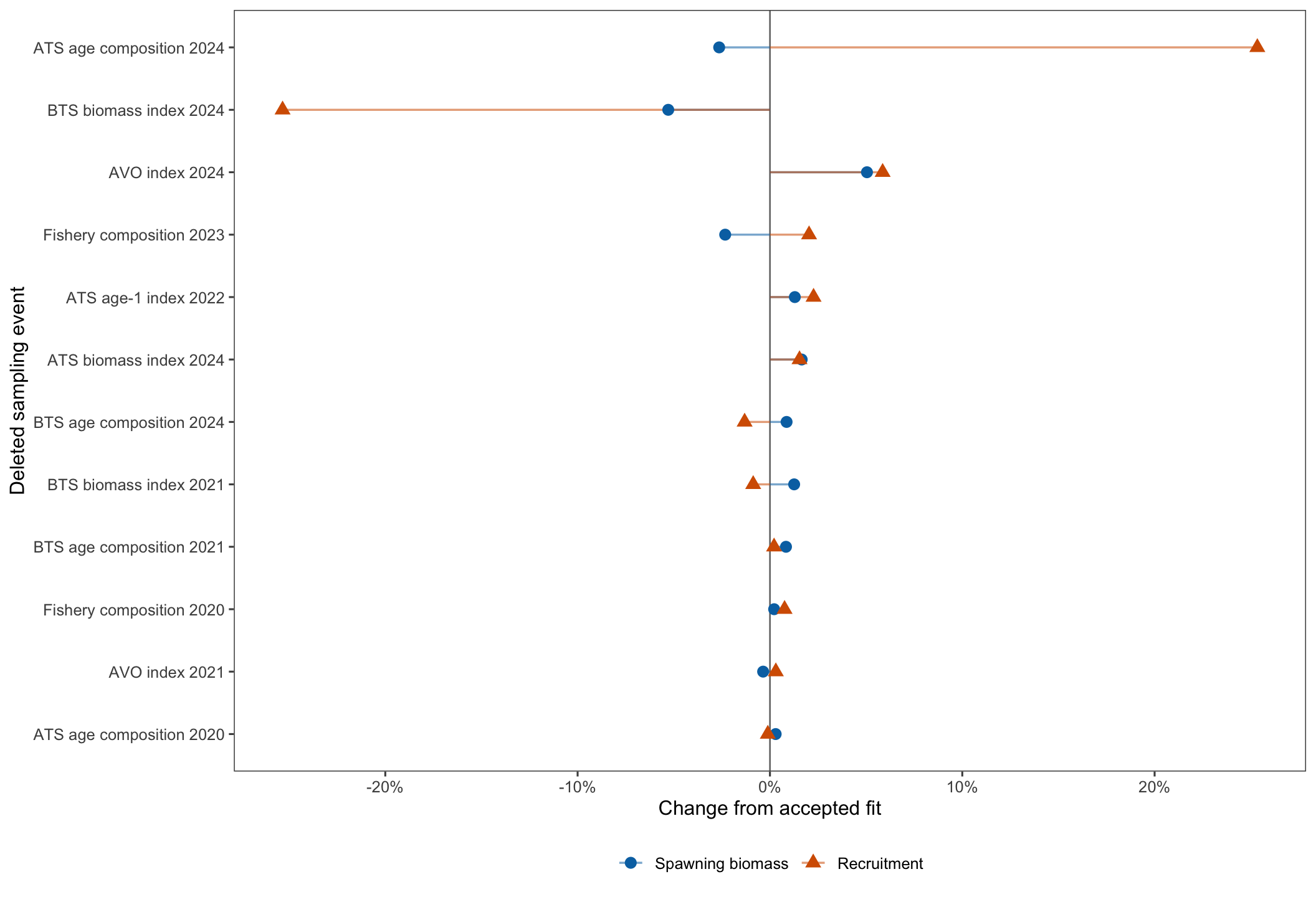
Across Figure 18 and Table 26, all 12 refits had status OK, positive-definite Hessians, and maximum absolute gradients below 8.2e-05. The largest terminal SSB response was -5.29% after deleting the 2024 BTS biomass index. The largest terminal recruitment responses were approximately 25.3% in opposite directions: lower without the 2024 BTS biomass index and higher without the 2024 ATS age composition. The largest recruitment response in any assessment year was 53.9%, for the 2023 recruitment estimate when the 2024 ATS age composition was removed. These are sensitivity measures, not evidence that an observation is erroneous or should be down-weighted.
| Deleted event | 2024 SSB change (percent) | 2024 recruitment change (percent) | Maximum recruitment change (percent) |
|---|---|---|---|
| Fishery composition 2020 | 0.22 | 0.76 | 14.50 |
| Fishery composition 2023 | −2.33 | 2.03 | 11.81 |
| BTS biomass index 2021 | 1.26 | −0.87 | 1.39 |
| BTS biomass index 2024 | −5.29 | −25.34 | 25.34 |
| BTS age composition 2021 | 0.83 | 0.21 | 7.48 |
| BTS age composition 2024 | 0.87 | −1.32 | 15.69 |
| ATS biomass index 2024 | 1.65 | 1.54 | 2.46 |
| ATS age composition 2020 | 0.30 | −0.11 | 0.33 |
| ATS age composition 2024 | −2.64 | 25.34 | 53.92 |
| ATS age-1 index 2022 | 1.29 | 2.27 | 8.64 |
| AVO index 2021 | −0.35 | 0.31 | 0.56 |
| AVO index 2024 | 5.04 | 5.86 | 9.79 |
The two strongest cases in Figure 18 and Table 26 were also refit from the saved full-data stage-A estimates. Their alternate and primary objectives differed by at most 1.4e-08, and their terminal changes agreed within 0.001 percentage points. This targeted check supports the numerical stability of the two largest reported effects.
The objective differences saved with these diagnostics are descriptive only: the fits contain different observations and the accepted stabilized composition objective is a pseudo-likelihood, so they are not likelihood-ratio tests. Formal PSIS-LOO remains a separate research task. It requires a proper grouped data density, a validated posterior sample, and conditional treatment of annual observations in the BTS covariance likelihood (Vehtari et al. 2017, 2024). The existing SparseNUTS analysis remains exploratory and is not used for assessment inference.
A-8 Acronyms
This appendix follows the glossary convention in the Alaska Stock Assessment Report (asar) package (Schiano et al. 2026). The project glossary uses ASAR’s \newacronym format and adds terms specific to this Rceattle comparison. The quoted label “PM” is a model name. The glossary defines the abbreviations used throughout the report (Table 27).
| Acronym | Definition |
|---|---|
| ADMB | AD Model Builder |
| AIC | Akaike information criterion |
| AR1 | first-order autoregressive |
| ATS | acoustic-trawl survey |
| AVO | acoustic vessels of opportunity |
| BTS | bottom trawl survey |
| CIE | Center for Independent Experts |
| CPUE | catch per unit effort |
| CSV | comma-separated values |
| DAG | directed acyclic graph |
| DSEM | dynamic structural equation modeling |
| ESP | ecosystem and socioeconomic profile |
| HTML | HyperText Markup Language |
| IID | independent and identically distributed |
| LOO | leave-one-out cross-validation |
| MCMC | Markov chain Monte Carlo |
| MVN | multivariate normal |
| OSA | one-step-ahead |
| PSIS | Pareto-smoothed importance sampling |
| RDS | R serialized data |
| RTMB | R Template Model Builder |
| SAFE | Stock Assessment and Fishery Evaluation |
| SDNR | standard deviation of normalized residuals |
| SEM | structural equation model |
| SPM | Standard Projection Model |
| SST | sea surface temperature |