Research and developments on the eastern Bering Sea walleye pollock stock assessment
September 2025, Plan Team Draft
1 Summary
This document is a follow-up to the discussion paper presented to the Center for Independent Experts (CIE) review panel prepared in May 2025 (link here; part 1 of this report). The review panel provided a set of recommendations to enhance the model structure, address key uncertainties, and improve transparency. This is Part 2 in which we show actions taken since the review and is intended inform the September 2025 NPFMC review. It focuses on migrating the operational model from ADMB to RTMB and begins to examine ways to evaluate the influence of the Russian fishery.
Since the May 2025 CIE review, several key developments have been made in the EBS pollock assessment. The most significant is the completed transition from ADMB to RTMB. The ported model successfully reproduces ADMB results for spawning biomass and recruitment with negligible differences, while enabling greater flexibility in estimating random-walk selectivity and recruitment deviations, propagating error through marginal likelihood, and integrating random effects. This provides a more modern and transparent framework for assessment. Work is also underway to address one of the reviewers’ main concerns—the absence of Russian removals. Scenario modeling is being conducted using Russian catch levels equivalent to 20–45% of U.S. catch, following reviewer guidance and recent publications. These runs will help bound the potential influence of transboundary removals before more collaborative modeling efforts are considered. Other areas highlighted by the review, such as process uncertainty, growth, weight-at-age, and alternative data-weighting approaches, remain planned or deferred. The tools for addressing them, including marginal-likelihood estimation of selectivity variance and Dirichlet–multinomial likelihoods, are now available in RTMB and other platforms, but implementation will follow the Russian catch work to avoid overlapping sources of change.
Bridging ADMB to RTMB required some adjustments in the ADMB code. These included shifting fishery dome-shaped selectivity penalties to apply at older ages and re-expressing “deviation-about-a-mean” parameterizations as direct level parameters with centered likelihoods. Verification exercises show that RTMB matches ADMB closely when fed identical parameter estimates, with gradients near zero and likelihood components in agreement. Importantly, RTMB’s integration with modern R tools also allows efficient Bayesian sampling, demonstrated with the adnuts R package.
Beyond model platform changes, comparative analyses were extended. Russian and U.S. assessments of pollock show broadly synchronous signals, particularly for recruitment, but differ markedly in scale: U.S. abundance estimates are typically two to four times greater than Russian estimates, with peaks exceeding fivefold differences in the early 2010s. These differences reflect not only survey coverage and model structure, but also contrasting harvest control rules. Russia has adopted a “modern MSY” approach, with higher target exploitation rates and lower biomass triggers, resulting in higher TACs when recruitment is favorable but greater risk if it falters. The U.S. maintains a more precautionary framework, constraining harvest below \(F_{MSY}\) and maintaining conservative biomass thresholds, which reduces volatility and risk. The immediate step to harmonize perspectives is the inclusion of Russian removals as a sensitivity analysis in the EBS assessment. A parallel comparison with the Gulf of Alaska pollock stock shows even starker contrasts, with EBS abundances five to fifteen times higher. Some weak coupling is evident at early ages, but overall the two populations are largely decoupled.
Additional technical notes were added for transparency, better documenting the form of first-difference selectivity penalties in both time and age and confirming lognormal survey likelihood formulations against ADMB. Looking forward, near-term priorities are clear: completing the Russian-catch sensitivity runs, testing marginal-likelihood estimation of selectivity variances, piloting Dirichlet–multinomial likelihoods, and preparing staged analyses of weight-at-age and potential time-varying natural mortality. The platform migration is complete and validated, and the largest remaining source of uncertainty for 2025 advice is the treatment of Russian removals, with process-error and likelihood improvements sequenced to follow that critical step.
2 Response to 2025 CIE Review of EBS Walleye Pollock Assessment
This section outlines the response to the findings and recommendations of the 2025 Center for Independent Experts (CIE) review of the Eastern Bering Sea (EBS) walleye pollock stock assessment. Links to the reviews can be found from Matt Cieri, Yan Jiao, and Anders Nielsen.
One of the reviewers’ primary concerns was the continued reliance on ADMB. This has now been resolved with the transition to RTMB, which enables easier use of random-effects for selectivity and recruitment deviations.
Another prominent theme was the absence of Russian removals from the assessment model. All three reviewers emphasized the need to explore the magnitude of this omission, both in terms of sensitivity runs and in better quantifying transboundary exchange. Work is in progress, with planned runs assuming Russian removals of 20–45% of U.S. catch based on (Japp and Sharov (2024)) and reviewer guidance. These scenarios will provide bounds on the possible scale of impacts before moving toward more collaborative or joint modeling approaches.
With respect to process uncertainty, selectivity, and growth, the reviewers identified several areas where additional flexibility could be valuable. Anders recommended estimating process variances for random-walk selectivity penalties using marginal likelihood, rather than fixing them. This aspect is possible within RCEATTLE and SPOCK currently, and is now available in the RTMB version of the pollock model (rpm). Yan noted that weight-at-age models could incorporate cohort and temperature effects, and also suggested cautious exploration of time-varying natural mortality, potentially informed by multispecies work such as CEATTLE. These issues have been partially addressed, and further exploration of process error variances will follow after the Russian catch work is integrated.
On data weighting and likelihood specification, Matt Cieri highlighted the potential advantages of a Dirichlet–multinomial (DM) framework and other benefits related to random effects estimation via the Laplace approximation. For now, the bootstrap-based effective sample size approach has been retained, with DM implementation available in three different platforms (RCEATTLE, SPOCK, and rpm). We anticipate examining this as an option in 2026 and seek guidance and advice from the Plan Teams and SSC.
A consolidated summary of reviewer recommendations and their current status is provided in Table 1.
| Theme | Lead Reviewer | Recommendation | Status |
|---|---|---|---|
| RTMB transition | All | Port model from ADMB to RTMB | ✅ Completed |
| Russian catch | All | Incorporate or test Russian removals | 🟡 In progress |
| Selectivity complexity | Nielsen | Estimate process variances via marginal likelihood | 🟡 In progress |
| Natural mortality | Jiao | Explore M variation and CEATTLE integration | 🟡 In progress |
| Growth & WAA | Jiao | Model cohort and temperature effects on WAA | ⚪ Deferred |
| Data weighting | Cieri | Test Dirichlet-multinomial likelihoods | ⚪ Available but deferred |
| Retrospective | Nielsen | Use Mohn's rho over shorter periods | ✅ Available |
Since the review, we ported the ADMB operational model used in 2024 to RTMB. We verified that outputs match the between versions. Secondly, we have taken initial steps to address the Russian catch uncertainty by comparing of assessments between regions.
3 Bridging ADMB to RTMB
The original ADMB code (first developed for application in 1996 (J. N. Ianelli and Fournier 1998)) has evolved over time and has a number of unique features. However, ADMB has less flexibility to incorporate random effects and marginal likelihood estimation. As such, we only adopted the set of features used for the 2024 EBS pollock assessment and fully ported those to RTMB. Features we ommitted included the ability to estimate time-varying natural mortality, predation and overlap factors, and a number of selectivity options to name a few. This transition enables several important enhancements, including the ability to estimate random-walk selectivity and recruitment deviations, improved error propagation through marginal likelihood, and greater transparency for code review and modifications.
We changed the ADMB code as little as possible to enable it to be compatible and work within the RTMB framework. One change was the use of an if statement in the penalty for dome-shaped selectivity in the fishery. In the original ADMB code, the penalty was invoked if the selectivity at one age was less than the selectivity at the previous adjacent younger age. The modification to this was simply to penalize log-selectivities of adjacent age groups older than age 6.
The ADMB code also has several cases where say \(y_i\) is a function of a parameter \(\theta\) and a deviation \(\epsilon_i\) such that \(y_i = \theta + \epsilon_i\). In ADMB, the deviations are estimated as a vector of parameters with a constraint to have mean zero., In RTMB, it seems best to reparameterize them as a simple vector of parameters (say as \(\theta_i\)) and then do the likelihood parts as deviations from the mean. To this end, we modified the original ADMB parameterization to from estimating a mean and time-varying deviations from that mean to simply a vector of values over time. These changes resulted in changes in the pattern of spawning biomass and recruitment estimates among the 2024 ADMB model and the 2024 modified version of the ADMB model used for comparisons with the RTMB results (Figure 1). We note that the main cause of the differences between the original ADMB and the modified ADMB is the change in the way the dome-shaped selectivity penalty is applied.
Show the code
library(ebswp)
library(patchwork)
pm_orig <- read_rep(here::here("runs", "lastyr", "pm.rep")) # Read in the report file)
pm_mod <- read_rep(here::here("runs", "rtmb", "pm.rep")) # Read in the report file)
sd_orig <- read_table(here::here("runs/lastyr", "pm.std")) |> filter(name=="pred_rec" )
sd_mod <- read_table(here::here("runs/rtmb", "pm.std"))|> filter(name=="pred_rec" )
df <- rbind( data.frame( name = "SSB",
value = as.numeric(pm_orig$SSB[,2]),
std.dev = as.numeric(pm_orig$SSB[,3]),
model = "ADMB original" ) ,
data.frame( name = "SSB",
value = as.numeric(pm_mod$SSB[,2]),
std.dev = as.numeric(pm_mod$SSB[,3]),
model = "ADMB Modified") )
df <- rbind(df, data.frame( name = "Recruits",
value = as.numeric(sd_orig$value),
std.dev = as.numeric(sd_orig$std.dev),
model = "ADMB original" ) ,
data.frame( name = "Recruits",
value = as.numeric(sd_mod$value),
std.dev = as.numeric(sd_mod$std.dev),
model = "ADMB Modified") )
df$Year <- rep(1964:2024, 4)
p1 <- df |> filter(name=="SSB",Year>1977) |>
ggplot(aes(x=Year, y=value, color=model)) + geom_point() + geom_line(aes(group=model)) +
geom_ribbon(aes(ymin=value-2*std.dev, ymax=value+2*std.dev, fill=model), alpha=0.2, color=NA) +
ggthemes::theme_few() + ylab("SSB (t)") + xlab("Year") +
scale_y_continuous(labels = scales::comma, limits=c(0,NA)) +
scale_x_continuous(breaks=seq(1965,2025,5))
p2 <- df |> filter(name=="Recruits", Year>1977) |>
ggplot(aes(x=as.factor(Year), y=value, color=model)) +
geom_point(size=2, position=position_dodge(width=0.8)) +
geom_errorbar(aes(ymin=value-2*std.dev, ymax=value+2*std.dev),
alpha=0.8, width=0.8, position=position_dodge(width=0.8)) +
ggthemes::theme_few() +
ylab("Age 1 Recruitment (thousands)") +
xlab("Year") +
scale_y_continuous(labels = scales::comma) +
expand_limits(y = 0) +
scale_x_discrete(breaks=seq(1980,2025,5))
p1/p2
3.1 RTMB Model implementation
For technical details on how one can re-code the pollock model into RTMB, the repository has R scripts that illustrate the approach used. In the R/ directory the main model code is in the file R/Rpm.R. The initial steps to bridge ADMB to RTMB involve identifying key components and their behaviors. We created a table function that was helpful to evaluate which components of the model in RTMB tracked with the ADMB version. When the bridging aspect was achieved there were extremely small differences between the two model versions (Table 2). Additionally, after some initial testing we were able to take the parameter estimates from the ADMB model and show that the gradients were very close to zero and the negative log-likelihood values matched (Table 3). The RTMB code was able to replicate the results from feeding the MLE parameter estimates from ADMB into the RTMB code (Figure 2). This gave virtually the same estimates of spawning stock biomass (SSB) and age 1 recruits (Figure 3).
Details of the RTMB implementation include initialization and parameter mapping contained in the R/config.R file. This file sources the required functions and libraries (including the model files R/Rpm.R, /R/utilities.R and R/model_funs.R. To facilitate the bridging, we retained all of the same parameters that were specified in the ADMB code (many of which are turned off as options for the model configuration). In order to mimic the “turning off” procedure done in ADMB, in RTMB they are simply “mapped” to be estimated or not. That is, for example if a model has 100 parameters specified in the code but only 80 are relevant given a model configuration, then in R the 20 parameters that are ommitted from estimation are given a value of NA. created a function rpm() that takes a vector of Initial estimation exercises (with “jittered” initial parameter values) suggested that the RTMB code required several re-starts to converge to the same solution as ADMB. We think this could be resolved by better phasing in of active parameters via the mapping procedure (similar to what is used in the ADMB code).
| Comparison of RTMB and ADMB Outputs | |||||
|---|---|---|---|---|---|
| Tolerance = 1e-05 | |||||
| Variable | Equal (≤ tol) | Length | Max |Abs diff| | Max |% diff| | Correlation |
| N | TRUE | 915 | 0.049919 | 0.000486 | 1.000000 |
| Z | TRUE | 915 | 0.000000 | 0.000161 | 1.000000 |
| F | TRUE | 915 | 0.000000 | 0.000482 | 1.000000 |
| M | TRUE | 915 | 0.000000 | 0.000000 | 1.000000 |
| S | TRUE | 915 | 0.000000 | 0.000123 | 1.000000 |
| pred_catch | TRUE | 61 | 0.004971 | 0.000383 | 1.000000 |
| obs_catch | TRUE | 61 | 0.005000 | 0.000458 | 1.000000 |
| SSB | TRUE | 61 | 0.004955 | 0.000447 | 1.000000 |
| phizero | TRUE | 1 | 0.000000 | 0.000189 | NA |
| Bzero | TRUE | 1 | 0.002409 | 0.000039 | NA |
| steepness | TRUE | 1 | 0.000000 | 0.000051 | NA |
| pred_cpue | TRUE | 12 | 0.004586 | 0.000146 | 1.000000 |
| pred_avo | TRUE | 18 | 0.000005 | 0.000409 | 1.000000 |
| eb_bts | TRUE | 42 | 0.048711 | 0.000456 | 1.000000 |
| eb_ats | TRUE | 19 | 0.004863 | 0.000244 | 1.000000 |
| sel_fsh | TRUE | 915 | 0.000005 | 0.000493 | 1.000000 |
| sel_bts | TRUE | 645 | 0.000000 | 0.000400 | 1.000000 |
| sel_ats | TRUE | 465 | 0.000005 | 0.000471 | 1.000000 |
| sam_fsh | TRUE | 60 | 0.000499 | 0.000134 | 1.000000 |
| sam_bts | TRUE | 42 | 0.000000 | 0.000000 | 1.000000 |
| sam_ats | TRUE | 19 | 0.000000 | 0.000000 | 1.000000 |
| phat_fsh | TRUE | 900 | 0.000000 | 0.000482 | 1.000000 |
| phat_bts | TRUE | 630 | 0.000000 | 0.000469 | 1.000000 |
| phat_ats | TRUE | 285 | 0.004855 | 0.000443 | 1.000000 |
| age_like | TRUE | 3 | 0.001047 | 0.000198 | 1.000000 |
| age_like_offset | TRUE | 3 | 0.039496 | 0.000326 | 1.000000 |
| cat_like | TRUE | 1 | 0.000002 | 0.000057 | NA |
| bts_like | TRUE | 1 | 0.000014 | 0.000043 | NA |
| ats_like | TRUE | 1 | 0.000002 | 0.000019 | NA |
| ats_age1_like | TRUE | 1 | 0.000024 | 0.000216 | NA |
| cpue_like | TRUE | 1 | 0.000003 | 0.000264 | NA |
| avo_like | TRUE | 1 | 0.000000 | 0.000004 | NA |
| avgsel_like | TRUE | 1 | 0.000000 | 0.000061 | NA |
| wt_nll | TRUE | 4 | 0.004116 | 0.000167 | 1.000000 |
| wt_like | TRUE | 1 | 0.004805 | 0.000076 | NA |
| rec_like | TRUE | 7 | 0.000042 | 0.000196 | 1.000000 |
| Fpen_like | TRUE | 1 | 0.000001 | 0.000015 | NA |
| sel_like | TRUE | 3 | 0.000021 | 0.000123 | 1.000000 |
| sel_like_dev | TRUE | 3 | 0.000464 | 0.000375 | 1.000000 |
| Priors | TRUE | 4 | 0.000024 | 0.000118 | 1.000000 |
| tot_like | TRUE | 1 | 0.004098 | 0.000052 | NA |
RPM) and the ADMB code results.
outer mgc: 6.36535e-06 outer mgc: 6.36535e-06
| Parameter | gradient |
|---|---|
| sel_slp_bts_dev | 6.365350e-06 |
| sel_devs_ats | -5.150768e-06 |
| sel_age_one_bts_dev | 4.980036e-06 |
| sel_devs_ats | 4.853937e-06 |
| sel_age_one_bts_dev | -4.486980e-06 |
| sel_slp_bts_dev | -4.402086e-06 |
| sel_devs_ats | 4.161281e-06 |
| sel_age_one_bts_dev | 4.138287e-06 |
| sel_devs_ats | -4.101133e-06 |
| sel_devs_ats | -4.097302e-06 |
| sel_slp_bts_dev | 3.487143e-06 |
| sel_slp_bts_dev | 3.258269e-06 |
| sel_devs_ats | 3.194401e-06 |
| sel_devs_ats | -3.190566e-06 |
| sel_devs_ats | 3.146215e-06 |
| sel_devs_ats | 3.068769e-06 |
| sel_devs_ats | 3.008710e-06 |
| sel_devs_ats | 2.963560e-06 |
| sel_age_one_bts_dev | 2.962122e-06 |
| sel_devs_ats | 2.952612e-06 |


3.2 RTMB implementation of MCMC integrations
A single run for a chain of 5,000 resulted in excellent mixing quality with the “poorest mixing” parameters demonstrating very good MCMC performance (Figure 4). The trace plots show the typical “fuzzy caterpillar” pattern indicating good mixing and the pairwise plots reveal appropriate exploration of parameter space. The chains appear to be sampling efficiently from the posterior distributions without any divergent transitions or other issues. The high effective sample size (ESS) values (ranging from ~900-1793) suggest that the chains are providing plenty of independent samples from the posterior distribution.
Using some of the additional features of the ADNUTS R package shows that in relatively few commands, a useful suite of diagnostics can be created (Figure 5).
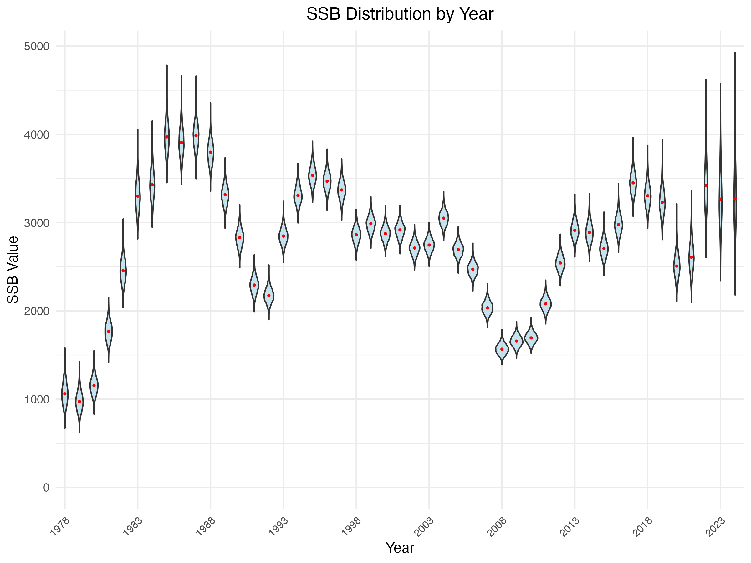
This figure provides comprehensive validation of the Bayesian MCMC results against frequentist asymptotic approximations for the EBS pollock stock assessment model, showing excellent overall performance across all diagnostics. Panel (a) demonstrates tight agreement between posterior standard deviations and asymptotic standard errors along the 1:1 line, validating that both approaches yield similar uncertainty estimates. Panel (b) shows well-behaved, approximately normal marginal posterior distributions for various log-scale parameters with good coverage by density curves, indicating proper sampling. Panel (c) presents the spawning stock biomass time series from 1978-2020, showing higher biomass in early years, decline through the 1980s-1990s, and lower variability in recent decades with appropriate uncertainty quantification throughout. Panel (d) displays pairwise plots for the 5 parameters with the greatest Bayesian-frequentist variance discrepancies, yet even these show reasonable correlations and good mixing in trace plots. Overall, this validation demonstrates that the RTMB Bayesian implementation performs excellently with close agreement to established frequentist methods while providing the additional benefits of full posterior distributions and proper uncertainty propagation.
The point of using MCMC’s is that in the future previously assumed variances can be estimated more objectively.


4 Considerations for future assessments regarding neighboring Russian federation fisheries
As this year’s assessment moves forward, particular attention is warranted on how Russian fisheries and assessments are considered alongside our own results. Pollock in the eastern and western Bering Sea are generally recognized as a single biological stock, with seasonal exchange across the U.S.–Russia boundary documented by acoustic studies. As noted in the CIE reviews, Russian removals are substantial with recent estimates representing on the order of 20–45% of the U.S. catch in some years. While examined in past assessments, the Russian catch magnitude should be re-evaluated to examine how they might alter management advice. As a step in beginning to make a more detailed evaluation, we compared the Russian stock assessment results presented as part of their Marine Stewardship Council (MSC) review panel with our model results (through 2024).
4.1 Comparison of Russian and USA age‑structured assessment results
Comparisons between Russian and U.S. assessments indicate that U.S. numbers-at-age are consistently higher, with total abundance estimates averaging about 2.9 times greater than Russian estimates (median ratio ≈ 2.7). Despite this scale difference, recruitment and biomass trends display synchrony, suggesting that both assessments capture shared population dynamics across the basin while differing in magnitude due to survey intensity, model structure, and management frameworks.
The comparison of U.S. and Russian pollock assessments shows that U.S. estimates of total numbers-at-age are consistently higher than those from Russia, typically by a factor of 2–4, with the ratio peaking above 5 in the early 2010s (Figure 6, bottom-left). Both assessments show similar interannual patterns, particularly for age-1 recruits (top-right), suggesting some shared signals of strong year classes. Correlation analysis by age class (bottom-right; Table 5) confirms this alignment, with moderate to strong positive correlations across ages 1–6. At older ages, correlations weaken and even turn negative (age 10), reflecting differences in how the two assessments treat age structure and fishery/survey data inputs. Overall, while the magnitude of estimates differs substantially between the two countries, the consistent synchrony in recruitment trends indicates that both assessments are capturing the same broad population dynamics, albeit with systematic differences in scale.
| Correlations between Russian and USA Age Classes | |
|---|---|
| Age | Correlation |
| 1 | 0.625 |
| 2 | 0.627 |
| 3 | 0.618 |
| 4 | 0.697 |
| 5 | 0.682 |
| 6 | 0.560 |
| 7 | 0.083 |
| 8 | 0.098 |
| 9 | 0.007 |
| 10 | −0.500 |


4.2 Comparison with the Gulf of Alaska (GOA) pollock estimates
Since the Russian context suggests some connectivity, for perspective, we thought it might be useful to conduct a similar comparison with results from the GOA pollock stock. Pollock assessments from the eastern Bering Sea (EBS) and Gulf of Alaska (GOA) show strong contrasts in both magnitude and dynamics of numbers-at-age. The EBS consistently supports far higher abundances across all ages and years (typically 5–15 times greater than the GOA; Figure 8). Recruitment pulses are evident in both regions, particularly at age 1, but the correlations by age class reveal only modest positive associations at younger ages, while older ages show little to no correspondence (Table 6). This indicates that early life stages may share some environmental drivers across basins, but overall population dynamics remain largely decoupled.
A more detailed breakdown by age class underscores these findings (Figure 9). Cohort strength in the EBS exhibits large variability with recurring strong year classes, while the GOA maintains lower overall abundance with weaker pulses. Time-series plots for ages 1–6 highlight this contrast, with the EBS showing sharp recruitment spikes and the GOA remaining more muted.
| Correlations between GOA and EBS Age Classes | |
|---|---|
| Age | Correlation |
| 1 | 0.321 |
| 2 | 0.324 |
| 3 | 0.289 |
| 4 | 0.264 |
| 5 | 0.200 |
| 6 | 0.162 |
| 7 | 0.142 |
| 8 | 0.071 |
| 9 | 0.032 |
| 10 | −0.064 |


In summary, the correlations between numbers at age from the GOA, EBS, and Russia are consistent with what has been observed from genetic studies and general movement of fish from the EBS into Russian waters (J. Ianelli et al. (2023), O’Leary et al. (2022), Levine et al. (2024))
5 Other items
The CIE noted in particular that some documentation of aspects of the ADMB code was incomplete. During the meetings, we began to more properly specify how the selectivity penalties were being calculated and implementated. These were identified and will be suplemented and corrected for the November documentation.
6 Plans for 2025 and beyond
For Council consideration in 2025 and beyond, we plan to continue with the 2024 model but with the updated bottom-trawl survey methods (as presented to the CIE see part 1 of this report).
For 2025 (this year) we will
adopt the updated software from AFSC GAP program to process the bottom-trawl survey data for aggregate biomass indices and age compositions (as presented to the CIE see part 1 of this report).
start with FT-NIR age compositions (processed in the same way as with results from traditional age estimation methods).
apply the revised estimates of acoustic-trawl survey uncertainty (as presented to the CIE see part 1 of this report; Urmy, Ressler, and De Robertis (2025)).
potentially continue to explore the use of the model converted to RTMB and run in parallel with the ADMB model (to the extent useful/practical).
If time allows, we will also explore some sensitivities with respect to the hypotheses on connectivity of the stock in adjacent Russian waters.
For 2026 we plan to:
Present as a replacement for the ADMB code the RTMB code presented here, or prefereably one of the models being developed in-house (Matt Cheng’s or Grant Adams’)
Continue to refine and validate the model structure, including selectivity pattern variability, random-effect factors affecting weight-at-age, and natural mortality rate variability.
Move forward with the FT-NIR age-composition data with fleet-specific age-error matrices
Further develop advancements of the previous work on integrating survey data from acoustics and bottom-trawl to better quantify variable patterns in the vertical distribution of pollock (Monnahan et al. (2021)).
Explore the potential for integrating data from Russian surveys (if feasible) and develop a spatially disaggregated model (2 or 3 areas) to better represent the population dynamics and connectivity of the stock across the Bering Sea and adjacent Russian waters.
Include some developments on diagnostics for models where the effective degrees of freedom can be estimated and provide improvements on the model selection criteria (e.g., AIC, BIC) for models with random effects (Zheng, Cadigan, and Thorson (2024)).