Compare {sdmgamindex} to regular GAMs
March 11 2024
C-model-comparisons.RmdGAMs: the old fashioned way
1. Wrangle Data
SPECIES <- c(# must match common name column
  "walleye pollock",
  "yellowfin sole",
  "red king crab"
)
YEARS <- 2015:2021
SRVY <- "EBS"
method <- "ML"
knotsP <- 376
# dir_out <- here::here("inst","regular_gam_approach")

crs_latlon = "+proj=longlat +datum=WGS84"
crs_proj = "EPSG:3338"

dat <- sdmgamindex::noaa_afsc_public_foss

# Get cold pool data using cold pool data from the {coldpool} R package
dat <- dat %>%
  dplyr::mutate(sx = ((longitude_dd_start - mean(longitude_dd_start, na.rm = TRUE))/1000),
                sy = ((latitude_dd_start - mean(latitude_dd_start, na.rm = TRUE))/1000)) %>%
  stats::na.omit() %>%
  dplyr::filter(common_name %in% SPECIES &
                  year %in% YEARS &
                  srvy %in% SRVY) %>%
  dplyr::rename(GEAR_TEMPERATURE = bottom_temperature_c,
                BOTTOM_DEPTH = depth_m,
                Year = year)

head(dat)
#>   Year srvy             survey survey_definition_id cruise cruisejoin haul
#> 1 2021  EBS eastern Bering Sea                   98 202101       -751   88
#> 2 2021  EBS eastern Bering Sea                   98 202101       -752   59
#> 3 2016  EBS eastern Bering Sea                   98 201601       -706   48
#> 4 2019  EBS eastern Bering Sea                   98 201901       -727   28
#> 5 2018  EBS eastern Bering Sea                   98 201801       -722   22
#> 6 2021  EBS eastern Bering Sea                   98 202101       -751   19
#>   hauljoin stratum station vessel_id   vessel_name           date_time
#> 1   -19996      20    L-01        94   VESTERAALEN 2021-06-21 15:21:16
#> 2   -19973      31    I-03       162 ALASKA KNIGHT 2021-06-14 12:10:16
#> 3   -15350      10    L-04        94   VESTERAALEN 2016-06-12 07:56:25
#> 4   -18780      31    B-08       162 ALASKA KNIGHT 2019-06-09 06:27:08
#> 5   -17559      31    I-12        94   VESTERAALEN 2018-06-06 12:32:44
#> 6   -19886      10    I-11        94   VESTERAALEN 2021-06-03 13:11:46
#>   latitude_dd_start longitude_dd_start latitude_dd_end longitude_dd_end
#> 1          58.65480          -167.8979        58.67117        -167.8579
#> 2          57.66072          -166.4836        57.66197        -166.5305
#> 3          58.64714          -165.9241        58.67214        -165.9363
#> 4          55.34481          -163.3904        55.34473        -163.4362
#> 5          57.65918          -160.9100        57.68333        -160.9030
#> 6          57.69411          -161.5022        57.66878        -161.5077
#>   GEAR_TEMPERATURE surface_temperature_c BOTTOM_DEPTH species_code  itis  worms
#> 1              3.7                   6.8           47        69322 97935 233889
#> 2              3.2                   5.7           67        69322 97935 233889
#> 3              6.5                   6.8           37        69322 97935 233889
#> 4              5.4                   8.7           53        69322 97935 233889
#> 5              4.1                   6.1           56        69322 97935 233889
#> 6              4.1                   5.7           53        69322 97935 233889
#>     common_name            scientific_name id_rank cpue_kgkm2 cpue_nokm2 count
#> 1 red king crab Paralithodes camtschaticus species   73.81732   43.11760     2
#> 2 red king crab Paralithodes camtschaticus species   69.57943   21.41565     1
#> 3 red king crab Paralithodes camtschaticus species   66.83110   70.34853     3
#> 4 red king crab Paralithodes camtschaticus species  127.86046   82.09339     4
#> 5 red king crab Paralithodes camtschaticus species  531.50033  274.20481    12
#> 6 red king crab Paralithodes camtschaticus species 1166.16772  964.34424    42
#>   weight_kg taxon_confidence area_swept_km2 distance_fished_km duration_hr
#> 1     3.424                1       0.046385              2.952       0.535
#> 2     3.249                1       0.046695              2.805       0.519
#> 3     2.850                1       0.042645              2.869       0.524
#> 4     6.230                1       0.048725              2.914       0.523
#> 5    23.260                1       0.043763              2.716       0.498
#> 6    50.790                1       0.043553              2.834       0.512
#>   net_width_m net_height_m performance           sx            sy
#> 1      15.713        2.299         0.0 0.0008104423  0.0004173062
#> 2      16.647        2.400         0.0 0.0022246523 -0.0005767738
#> 3      14.864        2.250         0.0 0.0027842223  0.0004096462
#> 4      16.721        2.244         6.3 0.0053179323 -0.0028926838
#> 5      16.113        3.144         0.0 0.0077982823 -0.0005783138
#> 6      15.368        2.572         0.0 0.0072060923 -0.0005433838
2. Formulas
fm <-  list(
  # Null model spatial and temporal with an additional year effect
  "fm_1_s_t_st" = "Year +
    s(sx,sy,bs=c('ts'),k=376) +
    s(sx,sy,bs=c('ts'),k=10,by=Year)",

  # Mdoel with simple covariates
  "fm_2_cov" =
    "s(BOTTOM_DEPTH,bs='ts',k=10) +
s(log(GEAR_TEMPERATURE+3),bs='ts',k=10)"
)
3. Run simple GAM models
Here are all of the models we want to try fitting:
comb <- tidyr::crossing(
  "SPECIES" = SPECIES,
  "fm_name" = gsub(pattern = " ", replacement = "_", x = names(fm))) %>%
  dplyr::left_join(
    x = .,
    y = data.frame("fm" = gsub(pattern = "\n", replacement = "",
                               x = unlist(fm), fixed = TRUE),
                   "fm_name" = gsub(pattern = " ", replacement = "_",
                                    x = names(fm))),
    by = "fm_name")

comb
#> # A tibble: 6 × 3
#>   SPECIES         fm_name     fm
#>   <chr>           <chr>       <chr>
#> 1 red king crab   fm_1_s_t_st Year +    s(sx,sy,bs=c('ts'),k=376) +     s(sx,sy…
#> 2 red king crab   fm_2_cov    s(BOTTOM_DEPTH,bs='ts',k=10) +s(log(GEAR_TEMPERAT…
#> 3 walleye pollock fm_1_s_t_st Year +    s(sx,sy,bs=c('ts'),k=376) +     s(sx,sy…
#> 4 walleye pollock fm_2_cov    s(BOTTOM_DEPTH,bs='ts',k=10) +s(log(GEAR_TEMPERAT…
#> 5 yellowfin sole  fm_1_s_t_st Year +    s(sx,sy,bs=c('ts'),k=376) +     s(sx,sy…
#> 6 yellowfin sole  fm_2_cov    s(BOTTOM_DEPTH,bs='ts',k=10) +s(log(GEAR_TEMPERAT…
models <- fittimes <- list()

for(i in 1:nrow(comb)){
  cat("Fitting ",comb$SPECIES[i],"\n", comb$fm_name[i], ": ", comb$fm[i], "\n")

  temp <- paste0(comb$SPECIES[i], " ", comb$fm_name[i])

  dat0 <- dat %>%
    dplyr::filter(common_name %in% comb$SPECIES[i])

  fittimes[[ temp ]] <-
    system.time ( models[[ temp ]] <-
                    gam(formula = as.formula(paste0("cpue_kgha ~ ", comb$fm[i])),
                        data = dat0,
                        family = tw,
                        gamma = 1.4)  )

}

save(models, fittimes, file = here::here("inst","VigC_model_output.rdata"))
4. Assess the model
b <- lapply(X = models, FUN = AIC)
bb <- sapply(models, `[`, 1)

# sdmgamindex::get_surveyidx_aic(models)

b <- AIC(models$`yellowfin sole fm_1_s_t_st`, models$`yellowfin sole fm_2_cov`)# get(paste0("b", 1:9))

b
#>                                            df      AIC
#> models$`yellowfin sole fm_1_s_t_st` 105.06470 13881.31
#> models$`yellowfin sole fm_2_cov`     15.22028 14558.49

# bb <- get(rownames(b)[b$AIC %in% min(b$AIC):(min(b$AIC)+5)])
# b$df %in% min(b$df):(min(b$df)+5)

# bb
bb <- models$`yellowfin sole fm_1_s_t_st`
# gam.check(bb)
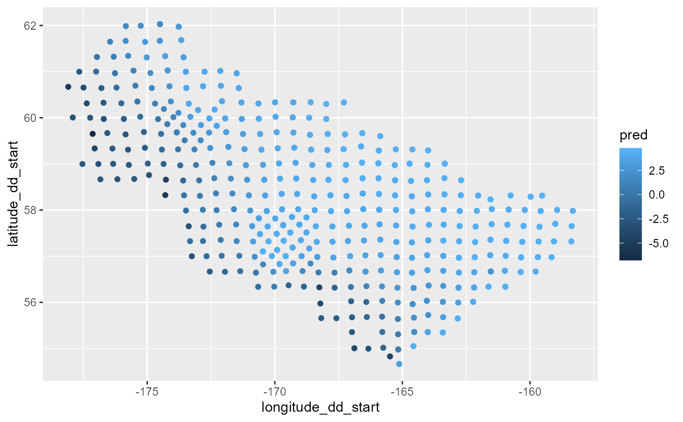
vis.gam(bb)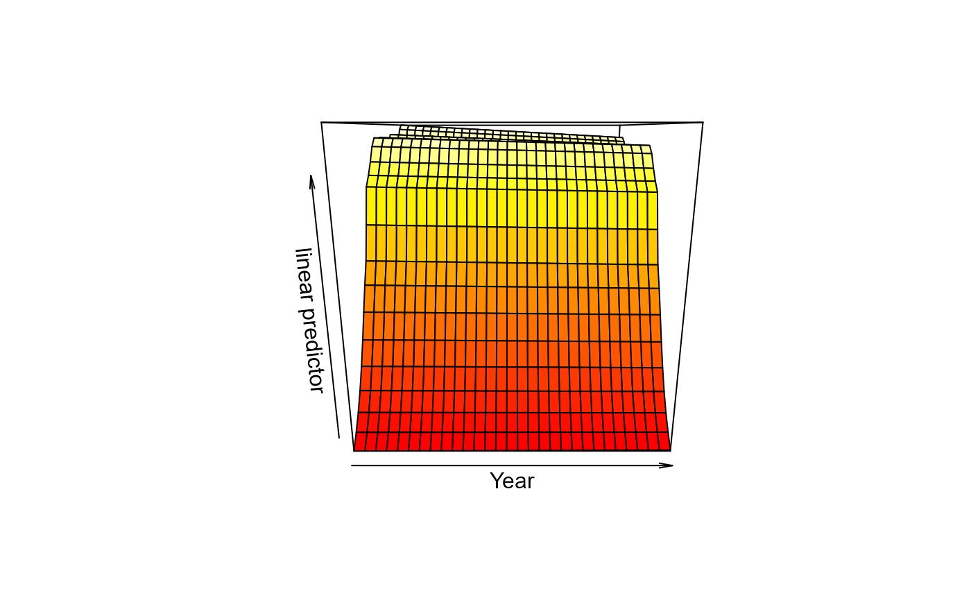
cc <- predict.gam(object = bb, newdata = dat[dat$Year == 2021,])

dat0 <- dat[dat$Year == 2021,] %>%
  dplyr::mutate(pred = cc)

figure <- ggplot() +
  geom_point(data = dat0,
             mapping = aes(x= longitude_dd_start, y = latitude_dd_start, color = pred))
figure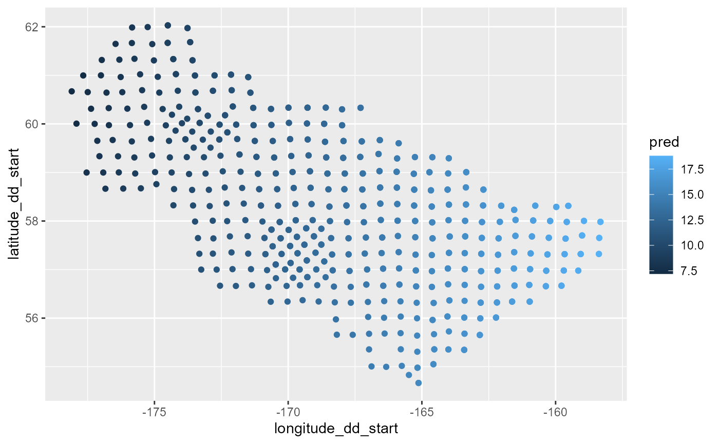
bb <- models$`yellowfin sole fm_2_cov`
# gam.check(bb)
vis.gam(bb)
cc <- predict.gam(object = bb, newdata = dat[dat$Year == 2021,])

dat0 <- dat[dat$Year == 2021,] %>%
  dplyr::mutate(pred = cc)

figure <- ggplot() +
  geom_point(data = dat0,
             mapping = aes(x= longitude_dd_start, y = latitude_dd_start, color = pred))
figure