{sdmgamindex} case study with and without covariates
March 11 2024
D-simple-case-study.RmdCheck your system:
sessionInfo()
#> R version 4.3.1 (2023-06-16 ucrt)
#> Platform: x86_64-w64-mingw32/x64 (64-bit)
#> Running under: Windows 10 x64 (build 19045)
#>
#> Matrix products: default
#>
#>
#> locale:
#> [1] LC_COLLATE=English_United States.utf8
#> [2] LC_CTYPE=English_United States.utf8
#> [3] LC_MONETARY=English_United States.utf8
#> [4] LC_NUMERIC=C
#> [5] LC_TIME=English_United States.utf8
#>
#> time zone: America/Los_Angeles
#> tzcode source: internal
#>
#> attached base packages:
#> [1] parallel  stats     graphics  grDevices utils     datasets  methods
#> [8] base
#>
#> other attached packages:
#>  [1] coldpool_3.3-1    viridis_0.6.5     stringr_1.5.1     reshape2_1.4.4
#>  [5] lubridate_1.9.3   fields_15.2       viridisLite_0.4.2 spam_2.10-0
#>  [9] ggthemes_5.1.0    akgfmaps_3.4.2    terra_1.7-71      stars_0.6-4
#> [13] abind_1.4-5       ggplot2_3.5.0     classInt_0.4-10   raster_3.6-26
#> [17] flextable_0.9.4   magrittr_2.0.3    gstat_2.1-1       dplyr_1.1.4
#> [21] DATRAS_1.01       sdmgamindex_0.1.1 tweedie_2.3.5     MASS_7.3-60.0.1
#> [25] sf_1.0-15         sp_2.1-3          RANN_2.6.1        marmap_1.0.10
#> [29] mapdata_2.3.1     maps_3.4.2        tidyr_1.3.1       mgcv_1.9-1
#> [33] nlme_3.1-164
#>
#> loaded via a namespace (and not attached):
#>  [1] rstudioapi_0.15.0       jsonlite_1.8.8          shape_1.4.6.1
#>  [4] rmarkdown_2.25          fs_1.6.3                ragg_1.2.7
#>  [7] vctrs_0.6.5             memoise_2.0.1           askpass_1.2.0
#> [10] htmltools_0.5.7         curl_5.2.1              sass_0.4.8
#> [13] KernSmooth_2.23-22      bslib_0.6.1             desc_1.4.3
#> [16] plyr_1.8.9              zoo_1.8-12              cachem_1.0.8
#> [19] uuid_1.2-0              igraph_2.0.2            mime_0.12
#> [22] lifecycle_1.0.4         pkgconfig_2.0.3         Matrix_1.6-5
#> [25] R6_2.5.1                fastmap_1.1.1           shiny_1.8.0
#> [28] digest_0.6.34           colorspace_2.1-0        rprojroot_2.0.4
#> [31] textshaping_0.3.7       RSQLite_2.3.5           fansi_1.0.6
#> [34] timechange_0.3.0        gdistance_1.6.4         compiler_4.3.1
#> [37] here_1.0.1              proxy_0.4-27            intervals_0.15.4
#> [40] bit64_4.0.5             fontquiver_0.2.1        withr_3.0.0
#> [43] DBI_1.2.2               openssl_2.1.1           icesDatras_1.4.1
#> [46] gfonts_0.2.0            tools_4.3.1             units_0.8-5
#> [49] zip_2.3.1               httpuv_1.6.14           glue_1.7.0
#> [52] promises_1.2.1          grid_4.3.1              generics_0.1.3
#> [55] gtable_0.3.4            class_7.3-22            data.table_1.15.2
#> [58] xml2_1.3.6              utf8_1.2.4              pillar_1.9.0
#> [61] later_1.3.2             splines_4.3.1           lattice_0.22-5
#> [64] FNN_1.1.4               bit_4.0.5               tidyselect_1.2.0
#> [67] fontLiberation_0.1.0    knitr_1.45              gridExtra_2.3
#> [70] fontBitstreamVera_0.1.1 crul_1.4.0              xfun_0.42
#> [73] adehabitatMA_0.3.16     stringi_1.8.3           yaml_2.3.8
#> [76] evaluate_0.23           codetools_0.2-19        httpcode_0.3.0
#> [79] officer_0.6.5           gdtools_0.3.7           tibble_3.2.1
#> [82] cli_3.6.2               xtable_1.8-4            systemfonts_1.0.5
#> [85] munsell_0.5.0           jquerylib_0.1.4         spacetime_1.3-1
#> [88] Rcpp_1.0.12             ellipsis_0.3.2          pkgdown_2.0.7
#> [91] blob_1.2.4              dotCall64_1.1-1         scales_1.3.0
#> [94] xts_0.13.2              e1071_1.7-14            ncdf4_1.22
#> [97] purrr_1.0.2             crayon_1.5.2            rlang_1.1.3
Case study
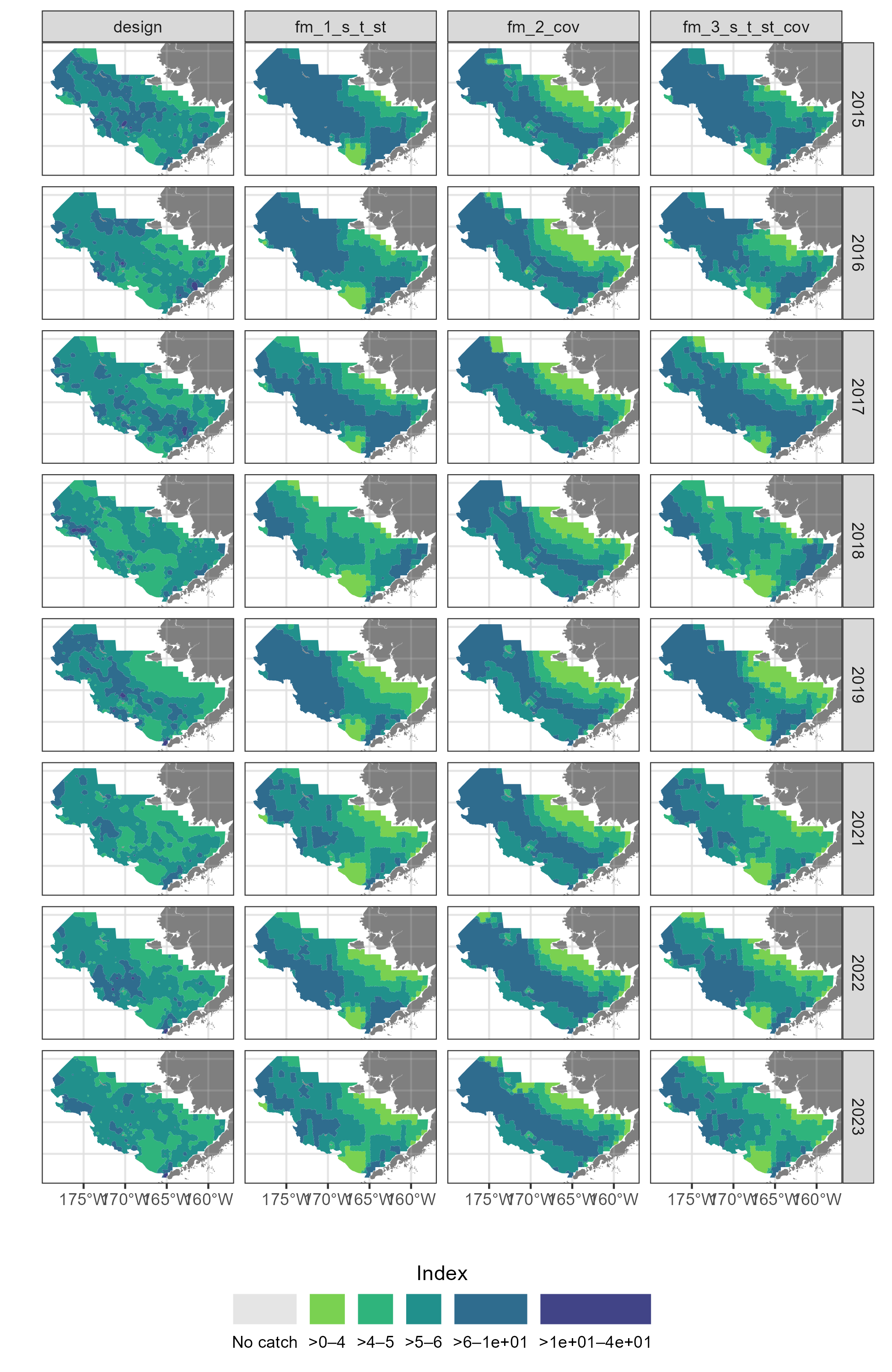
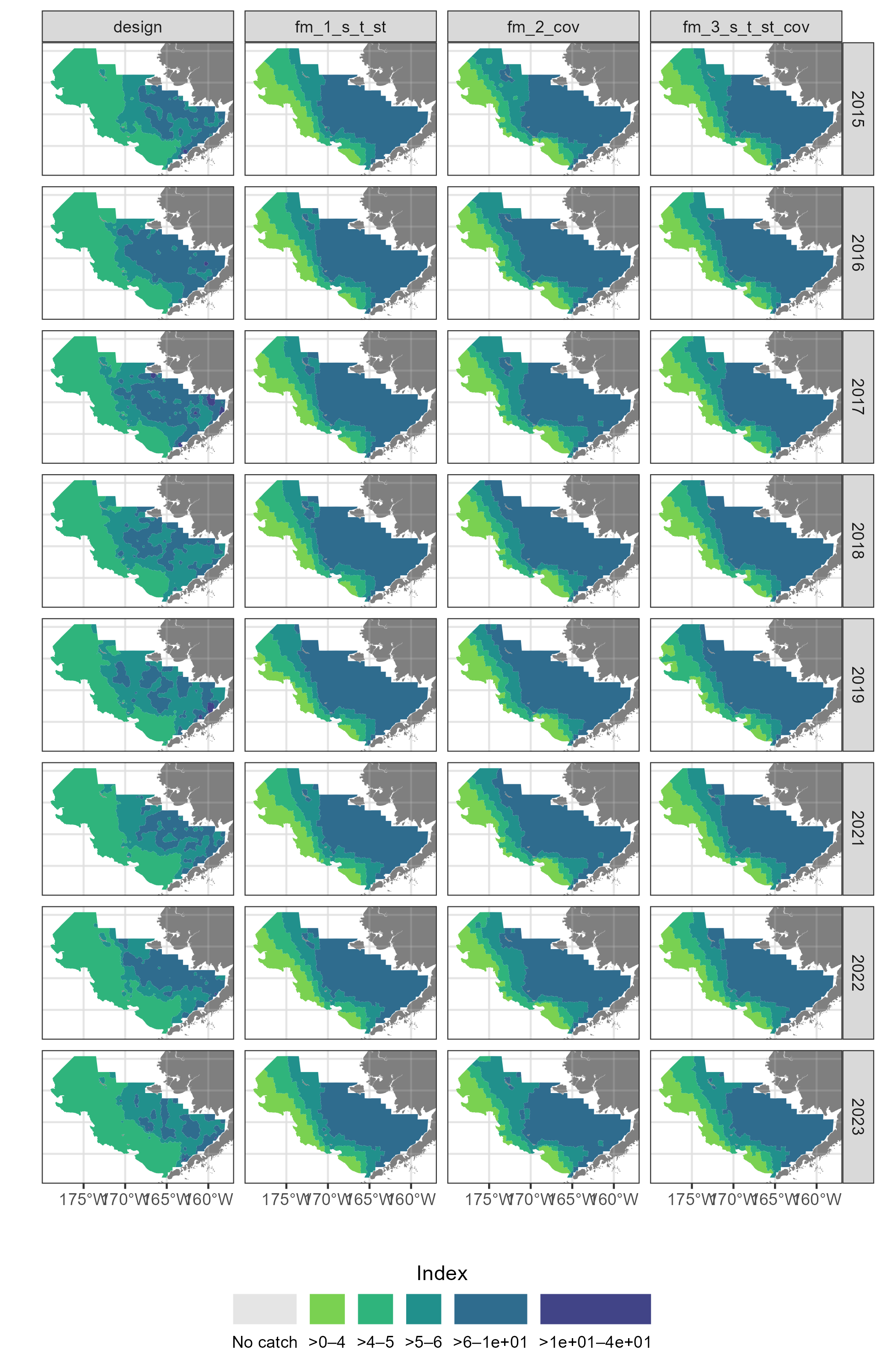
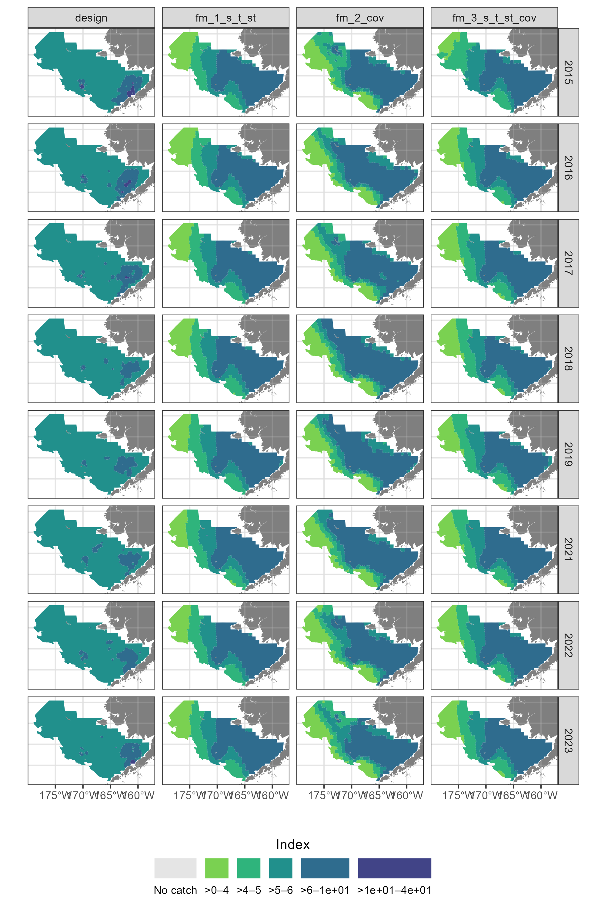
In this example, we will use data from NOAA Fisheries’ eastern Bering sea (EBS) bottom trawl survey. The Resource Assessment and Conservation Engineering (RACE) Division Groundfish Assessment Program (GAP) of the Alaska Fisheries Science Center (AFSC) conducts fisheries-independent bottom trawl surveys to assess the populations of demersal fish and crab stocks of Alaska. The species covered in this case study include yellow fin sole, walleye pollock, and red king crab.
|
Yellowfin Sole |
|
Walleye pollock |
|
Red King Crab |


And we are going to estimate the indicies of these species Over the eastern and northern Bering Sea shelf.
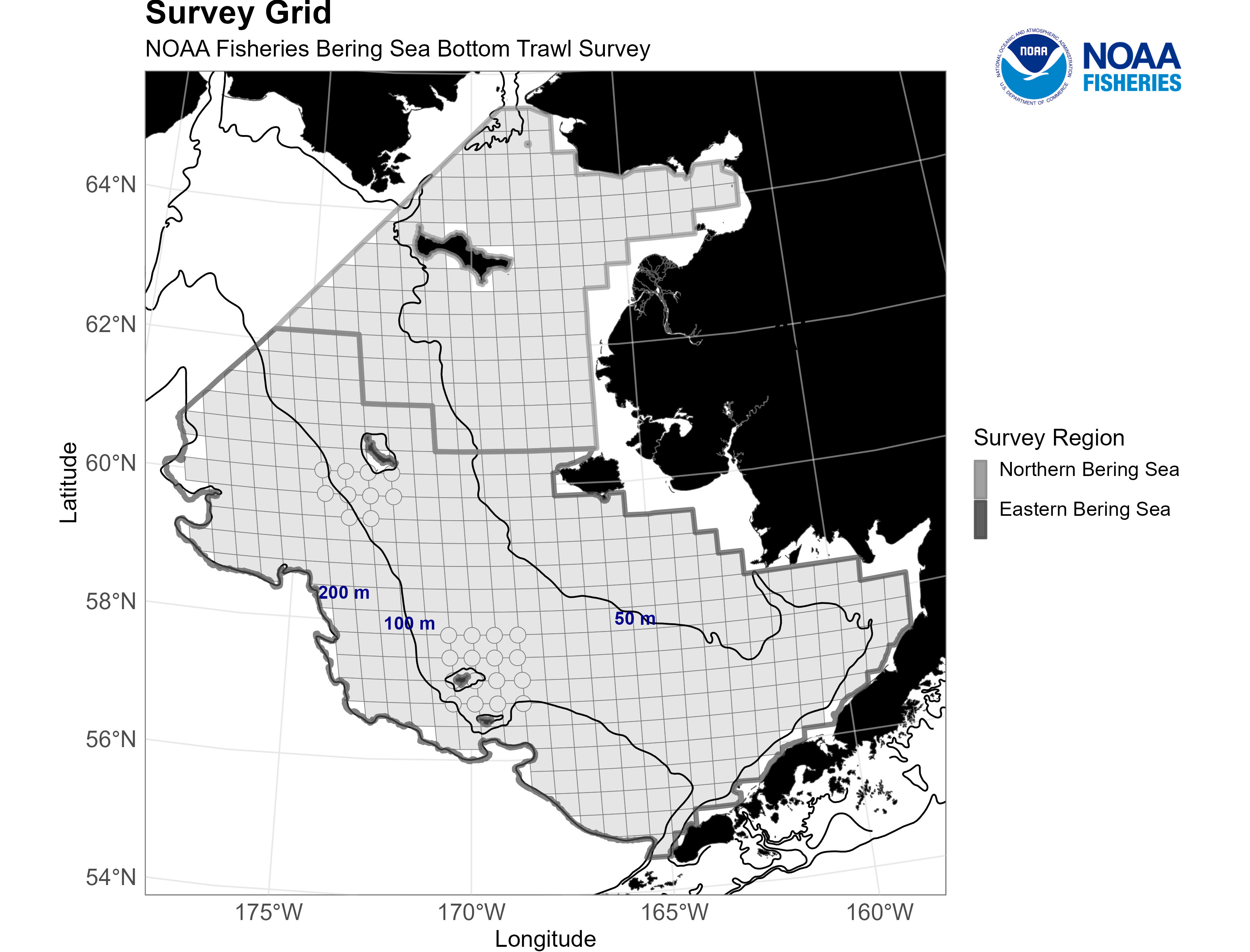
The grid of designated stations in the eastern Bering Sea and northern Bering Sea bottom trawl survey areas as well as the 50m, 100m, and 200m bathymetric boundaries. Credit: NOAA Fisheries
For the sake of a simple example, we will only assess data from 2015 to 2021.
SPECIES <- c("yellowfin sole", "walleye pollock", "red king crab")
YEARS <- 2015:2023
SRVY <- "EBS"
1. What data area we using?
Here, we use the public facing data from the NOAA AFSC groundfish Bering sea bottom trawl survey. For more information about how these data were compiled, see afsc-gap-products GitHub repo.
dat <- sdmgamindex::noaa_afsc_public_foss %>%
  dplyr::filter(srvy == SRVY &
                  year %in% YEARS &
                  common_name %in% SPECIES) %>%
  dplyr::mutate(hauljoin = paste0(stratum, "_", station, "_", date_time)) %>%
  dplyr::select(
    year, date_time, latitude_dd_start, longitude_dd_start, # spatiotemproal data
    cpue_kgkm2, common_name, # catch data
    bottom_temperature_c, depth_m, # possible covariate data
    srvy, area_swept_km2, duration_hr, vessel_id, hauljoin # haul/effort data)
  )
table(dat$common_name)
#>
#>   red king crab walleye pollock  yellowfin sole
#>            3008            3008            3008
head(dat)
#>   year           date_time latitude_dd_start longitude_dd_start cpue_kgkm2
#> 1 2023 2023-07-09 07:27:45          56.65940          -171.3599    0.00000
#> 2 2023 2023-07-09 07:51:03          56.99770          -173.2508    0.00000
#> 3 2023 2023-07-01 07:06:31          57.67576          -170.2871  419.72701
#> 4 2023 2023-06-18 12:58:27          58.00859          -166.5287   79.13648
#> 5 2022 2022-07-24 07:39:26          60.02075          -176.7193    0.00000
#> 6 2022 2022-07-23 16:59:28          59.32891          -177.0694    0.00000
#>     common_name bottom_temperature_c depth_m srvy area_swept_km2 duration_hr
#> 1 red king crab                  4.1     119  EBS       0.049888       0.504
#> 2 red king crab                  4.0     142  EBS       0.049980       0.509
#> 3 red king crab                  2.3      73  EBS       0.049842       0.515
#> 4 red king crab                  0.3      61  EBS       0.049939       0.530
#> 5 red king crab                  2.0     141  EBS       0.052054       0.548
#> 6 red king crab                  2.9     150  EBS       0.054499       0.539
#>   vessel_id                    hauljoin
#> 1       134 61_F-23_2023-07-09 07:27:45
#> 2       162 61_G-26_2023-07-09 07:51:03
#> 3       134 42_I-21_2023-07-01 07:06:31
#> 4       134 31_J-03_2023-06-18 12:58:27
#> 5        94 61_P-30_2022-07-24 07:39:26
#> 6       162 61_N-31_2022-07-23 16:59:28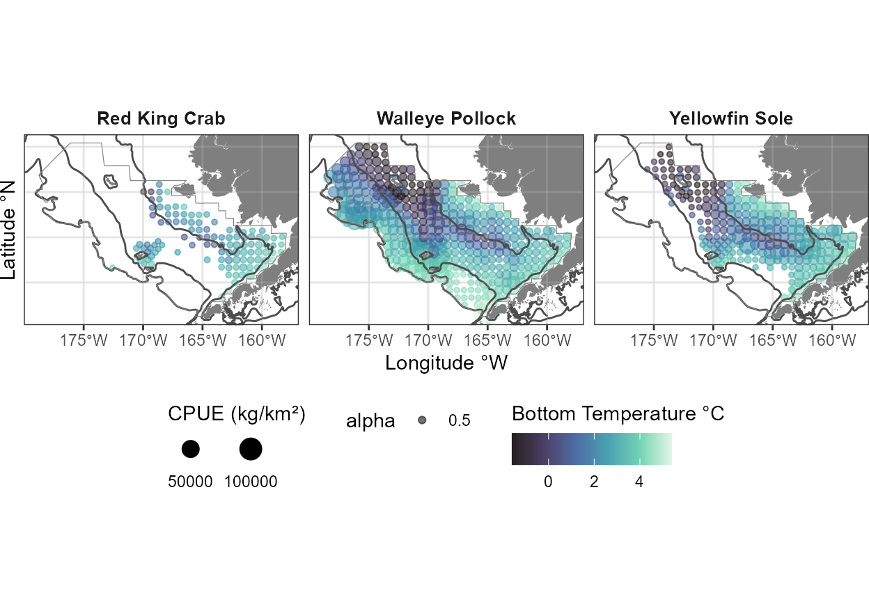
2023 species distribution relative densities (size) and bottom temperature (color).
2. Prepare the data from sdmgamindex::get_surveyidx():
# project spatial data
crs_proj <- "EPSG:3338" # NAD83 / Alaska Albers
crs_latlon <- "+proj=longlat +datum=WGS84" # decimal degrees

ll <- sdmgamindex::convert_crs(
  x = dat$longitude_dd_start,
  y = dat$latitude_dd_start,
  crs_in = crs_latlon,
  crs_out = crs_proj)

YEARS <- sort(unique(dat$year))

# The sdmgamindex::get_surveyidx() expects some columns to be named in a specific way
dat_wrangled <- dat %>%
  dplyr::rename(
    Year = year,
    wCPUE = cpue_kgkm2,
    COMMON_NAME = common_name,
    GEAR_TEMPERATURE = bottom_temperature_c,
    BOTTOM_DEPTH = depth_m,
    HaulDur = duration_hr,
    EFFORT = area_swept_km2,
    Ship = vessel_id) %>%
  dplyr::mutate(
    # create some other vars
    Lon = longitude_dd_start,
    Lat = latitude_dd_start,
    lon = ll$X,
    lat = ll$Y,
    sx = ((longitude_dd_start - mean(longitude_dd_start, na.rm = TRUE))/1000),
    sy = ((latitude_dd_start - mean(latitude_dd_start, na.rm = TRUE))/1000),
    ctime = as.numeric(as.character(Year)),
    date_time = as.Date(x = date_time, format = "%m/%d/%Y %H:%M:%S"),
    hour = as.numeric(format(date_time,"%H")),
    minute = as.numeric(format(date_time,"%M")),
    day = as.numeric(format(date_time,"%d")),
    month = as.numeric(format(date_time,"%m")),
    TimeShotHour = hour + minute/60,
    timeOfYear = (month - 1) * 1/12 + (day - 1)/365,

    # add some dummy vars and create some other vars
    Country = "USA",
    Gear = "dummy",
    Quarter = "2")  %>%
  dplyr::mutate(across((c("Year", "Ship", "COMMON_NAME")), as.factor)) %>%
  dplyr::select(wCPUE, GEAR_TEMPERATURE, BOTTOM_DEPTH, COMMON_NAME, EFFORT,
                Year, Ship, Lon, Lat, lat, lon, sx, sy,
                ctime, TimeShotHour, timeOfYear, Gear, Quarter, HaulDur, hauljoin)
head(dat_wrangled)
#>       wCPUE GEAR_TEMPERATURE BOTTOM_DEPTH   COMMON_NAME   EFFORT Year Ship
#> 1   0.00000              4.1          119 red king crab 0.049888 2023  134
#> 2   0.00000              4.0          142 red king crab 0.049980 2023  162
#> 3 419.72701              2.3           73 red king crab 0.049842 2023  134
#> 4  79.13648              0.3           61 red king crab 0.049939 2023  134
#> 5   0.00000              2.0          141 red king crab 0.052054 2022   94
#> 6   0.00000              2.9          150 red king crab 0.054499 2022  162
#>         Lon      Lat       lat        lon           sx            sy ctime
#> 1 -171.3599 56.65940  877146.6 -1050529.3 -0.002601332 -0.0016013454  2023
#> 2 -173.2508 56.99770  944820.3 -1151106.0 -0.004492212 -0.0012630454  2023
#> 3 -170.2871 57.67576  970747.6  -959416.2 -0.001528562 -0.0005849854  2023
#> 4 -166.5287 58.00859  959133.7  -734085.4  0.002229868 -0.0002521554  2023
#> 5 -176.7193 60.02075 1328406.2 -1237677.9 -0.007960682  0.0017600046  2022
#> 6 -177.0694 59.32891 1262236.5 -1282319.2 -0.008310772  0.0010681646  2022
#>   TimeShotHour timeOfYear  Gear Quarter HaulDur                    hauljoin
#> 1            0  0.5219178 dummy       2   0.504 61_F-23_2023-07-09 07:27:45
#> 2            0  0.5219178 dummy       2   0.509 61_G-26_2023-07-09 07:51:03
#> 3            0  0.5000000 dummy       2   0.515 42_I-21_2023-07-01 07:06:31
#> 4            0  0.4632420 dummy       2   0.530 31_J-03_2023-06-18 12:58:27
#> 5            0  0.5630137 dummy       2   0.548 61_P-30_2022-07-24 07:39:26
#> 6            0  0.5602740 dummy       2   0.539 61_N-31_2022-07-23 16:59:28
3. Define representitive station points to fit and predict the model at
Since surveys are not done at the same exact location each year (it’s the intention, but impossible in practice), we need to define what representative latitudes and longitudes we are going to predict at.
These are the same prediction grids AFSC uses for their 2021 VAST model-based indices (which is subject to change - do not use this without asking/checking that this is still current!).
pred_grid <- sdmgamindex::pred_grid_ebs

ll <- sdmgamindex::convert_crs(
  x = pred_grid$lon,
  y = pred_grid$lat,
  crs_in = crs_latlon,
  crs_out = crs_proj)

pred_grid <- pred_grid %>%
  dplyr::mutate(
    lon = ll$X,
    lat = ll$Y,
    sx = ((lon - mean(lon, na.rm = TRUE))/1000),
    sy = ((lat - mean(lat, na.rm = TRUE))/1000))

head(pred_grid)
#> # A tibble: 6 × 5
#>         lon      lat Shape_Area    sx    sy
#>       <dbl>    <dbl>      <dbl> <dbl> <dbl>
#> 1 -1133214. 1542340.   2449160. -290.  517.
#> 2 -1129510. 1542340.   9298535. -287.  517.
#> 3 -1125806. 1542340.   9749166. -283.  517.
#> 4 -1122102. 1542340.   5383834. -279.  517.
#> 5 -1118398. 1542340.   1173734. -275.  517.
#> 6 -1140622. 1538636.   1525663. -298.  513.
It is also good to have a shapefile on hand to crop and constrain your outputs too. Here at AFSC GAP, we have developed the {akgfmaps} R package to save and share such shapefiles.
# library(devtools)
# devtools::install_github("afsc-gap-products/akgfmaps", build_vignettes = TRUE)
library(akgfmaps)

map_layers <- akgfmaps::get_base_layers(
  select.region = "bs.south",
  set.crs = crs_proj)

# Let's just see what that looks like:
tmp <- map_layers$survey.area
tmp$AREA_KM2 <- tmp$PERIM_KM <- NULL

plot(tmp)
4. Prepare covariate data
Here we want to match covariate data to the prediction grid.
dat_cov <- sdmgamindex::pred_grid_ebs %>%
  dplyr::select(-Shape_Area) %>%
  dplyr::mutate(
    sx = ((lon - mean(lon, na.rm = TRUE))/1000),
    sy = ((lat - mean(lat, na.rm = TRUE))/1000))

sp_extrap_raster <- SpatialPoints(
  coords = coordinates(as.matrix(dat_cov[,c("lon", "lat")])),
  proj4string = CRS(crs_latlon) )
dat_cov
#> # A tibble: 36,690 × 4
#>      lon   lat       sx      sy
#>    <dbl> <dbl>    <dbl>   <dbl>
#>  1 -176.  62.1 -0.00748 0.00384
#>  2 -176.  62.1 -0.00741 0.00385
#>  3 -176.  62.2 -0.00735 0.00386
#>  4 -176.  62.2 -0.00728 0.00387
#>  5 -176.  62.2 -0.00721 0.00389
#>  6 -176.  62.1 -0.00759 0.00379
#>  7 -176.  62.1 -0.00752 0.00380
#>  8 -176.  62.1 -0.00746 0.00381
#>  9 -176.  62.1 -0.00739 0.00382
#> 10 -176.  62.1 -0.00732 0.00383
#> # ℹ 36,680 more rows
sp_extrap_raster
#> class       : SpatialPoints
#> features    : 36690
#> extent      : -178.9664, -157.9516, 54.48348, 62.19158  (xmin, xmax, ymin, ymax)
#> crs         : +proj=longlat +datum=WGS84 +no_defs
4a. Data that varies over only space (depth)
Here in the Bering sea, the depth rarely changes. The modeler may consider making this variable time-varying as well if they are say, in the Gulf of Alaska or the Aleutian Islands where currents and island formation can markedly change depth.
For this, we are going to create a raster of depth in the Bering sea from the survey data so we can merge that into the dataset at the prediction grid lat/lons.
x <- dat_wrangled %>%
  dplyr::select(Lon, Lat, BOTTOM_DEPTH) %>%
  stats::na.omit()  %>%
  sf::st_as_sf(x = .,
               coords = c(x = "Lon", y = "Lat"),
               crs = sf::st_crs(crs_latlon))

idw_fit <- gstat::gstat(formula = BOTTOM_DEPTH ~ 1,
                        locations = x,
                        nmax = 4)

# stn_predict <- raster::predict(idw_fit, x)

extrap_data0 <- raster::predict(
  idw_fit, sp_extrap_raster) %>%
  # as(sp_extrap_raster, Class = "SpatialPoints")) %>%
  sf::st_as_sf() %>%
  sf::st_transform(crs = crs_latlon)  %>%
  stars::st_rasterize()

extrap_data <- stars::st_extract(x = extrap_data0,
                                 at = as.matrix(dat_cov[,c("lon", "lat")]))

# to make future runs of this faster:
save(extrap_data0, extrap_data,
     file = here::here("inst",
                       paste0("vigD_bottom_depth_raster_",
                              min(YEARS),"-",max(YEARS), ".rdata")))
# Just so we can see what we are looking at:
plot(extrap_data0, main = "Interpolated Bottom Depths") 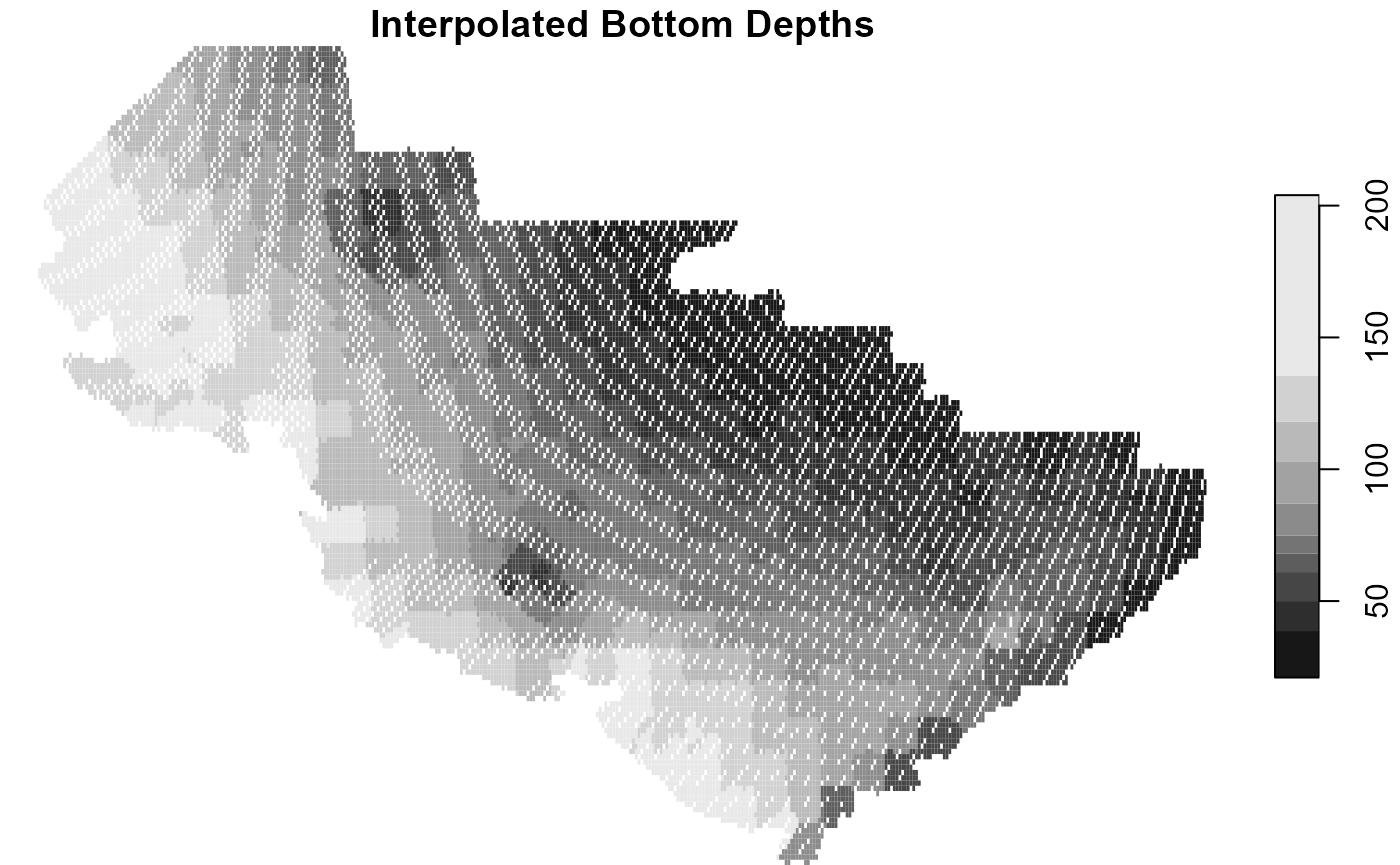
dat_cov <- cbind.data.frame(dat_cov,
                            "BOTTOM_DEPTH" = extrap_data$var1.pred) %>%
  stats::na.omit()

head(dat_cov)
#>         lon      lat           sx          sy BOTTOM_DEPTH
#> 1 -176.2068 62.13518 -0.007481089 0.003842524     93.00000
#> 2 -176.1395 62.14603 -0.007413772 0.003853379     93.00000
#> 3 -176.0722 62.15686 -0.007346407 0.003864203     93.00000
#> 4 -176.0047 62.16765 -0.007278995 0.003874995     92.76145
#> 5 -175.9373 62.17841 -0.007211535 0.003885756     92.75523
#> 6 -176.3179 62.08210 -0.007592106 0.003789448     93.00000
4b. Data that varies over space and time (bottom temperature)
Here, bottom temperature, and thereby the cold pool extent, have been show to drive the distribution of many species. This is especially true for walleye pollock.
For this we are going to lean on our in-house prepared validated and pre-prepared {coldpool} R package [@RohanColdPool]. This data interpolates over the whole area of the survey so there are no missing data.
# Just so we can see what we are looking at:
#plot(terra::unwrap(coldpool::ebs_bottom_temperature))
tmp <- which(readr::parse_number(names(terra::unwrap(coldpool::ebs_bottom_temperature))) %in% YEARS)

dat_temperature <- terra::unwrap(coldpool::ebs_bottom_temperature)[[tmp]] %>%
  terra::extract(y = dat_cov[,c("lon", "lat")] %>%
                   sf::sf_project(from = "+proj=longlat",
                                  to = "EPSG:3338")) %>%
  data.frame()
names(dat_temperature) <- paste0("GEAR_TEMPERATURE", YEARS)

dat_cov <- dplyr::bind_cols(dat_cov, dat_temperature) %>%
  na.omit()
head(dat_cov)
#>         lon      lat           sx          sy BOTTOM_DEPTH GEAR_TEMPERATURE2015
#> 2 -176.1395 62.14603 -0.007413772 0.003853379     93.00000          -0.07311002
#> 3 -176.0722 62.15686 -0.007346407 0.003864203     93.00000          -0.07311002
#> 4 -176.0047 62.16765 -0.007278995 0.003874995     92.76145          -0.15166534
#> 7 -176.2507 62.09301 -0.007524943 0.003800355     93.00000           0.06603578
#> 8 -176.1835 62.10389 -0.007457733 0.003811231     93.00000          -0.02377643
#> 9 -176.1162 62.11473 -0.007390475 0.003822076     93.00000          -0.11071504
#>   GEAR_TEMPERATURE2016 GEAR_TEMPERATURE2017 GEAR_TEMPERATURE2018
#> 2          -0.30315974            0.2442329             2.066675
#> 3          -0.30315974            0.2442329             2.066675
#> 4          -0.40172631            0.1406713             2.046152
#> 7          -0.08488923            0.4213759             2.109732
#> 8          -0.18901448            0.3380764             2.087453
#> 9          -0.29478970            0.2444835             2.064520
#>   GEAR_TEMPERATURE2019 GEAR_TEMPERATURE2021 GEAR_TEMPERATURE2022
#> 2             1.242070            0.1678221           -1.1127377
#> 3             1.242070            0.1678221           -1.1127377
#> 4             1.178158            0.1119230           -1.1903751
#> 7             1.372879            0.3057251           -0.9713215
#> 8             1.317465            0.2446349           -1.0861878
#> 9             1.257273            0.1832289           -1.1890295
#>   GEAR_TEMPERATURE2023
#> 2           -0.9886659
#> 3           -0.9886659
#> 4           -1.0962228
#> 7           -0.7410921
#> 8           -0.8782412
#> 9           -1.0114685
5. DATRAS structure
5a. Catch Data
# Identify vars that will be used --------------------------------------------
varsbyyr <- unique( # c("GEAR_TEMPERATURE", "cpi")
  gsub(pattern = "[0-9]+",
       replacement = "",
       x = names(dat_cov)[grepl(names(dat_cov),
                                pattern = "[0-9]+")]))

vars <- unique( # c("BOTTOM_DEPTH")
  names(dat_cov)[!grepl(names(dat_cov),
                        pattern = "[0-9]+")])
vars <- vars[!(vars %in% c("LONG", "LAT", "lon", "lat", "sx", "sy"))]

dat_catch_haul <- dat_wrangled
head(dat_catch_haul)
#>       wCPUE GEAR_TEMPERATURE BOTTOM_DEPTH   COMMON_NAME   EFFORT Year Ship
#> 1   0.00000              4.1          119 red king crab 0.049888 2023  134
#> 2   0.00000              4.0          142 red king crab 0.049980 2023  162
#> 3 419.72701              2.3           73 red king crab 0.049842 2023  134
#> 4  79.13648              0.3           61 red king crab 0.049939 2023  134
#> 5   0.00000              2.0          141 red king crab 0.052054 2022   94
#> 6   0.00000              2.9          150 red king crab 0.054499 2022  162
#>         Lon      Lat       lat        lon           sx            sy ctime
#> 1 -171.3599 56.65940  877146.6 -1050529.3 -0.002601332 -0.0016013454  2023
#> 2 -173.2508 56.99770  944820.3 -1151106.0 -0.004492212 -0.0012630454  2023
#> 3 -170.2871 57.67576  970747.6  -959416.2 -0.001528562 -0.0005849854  2023
#> 4 -166.5287 58.00859  959133.7  -734085.4  0.002229868 -0.0002521554  2023
#> 5 -176.7193 60.02075 1328406.2 -1237677.9 -0.007960682  0.0017600046  2022
#> 6 -177.0694 59.32891 1262236.5 -1282319.2 -0.008310772  0.0010681646  2022
#>   TimeShotHour timeOfYear  Gear Quarter HaulDur                    hauljoin
#> 1            0  0.5219178 dummy       2   0.504 61_F-23_2023-07-09 07:27:45
#> 2            0  0.5219178 dummy       2   0.509 61_G-26_2023-07-09 07:51:03
#> 3            0  0.5000000 dummy       2   0.515 42_I-21_2023-07-01 07:06:31
#> 4            0  0.4632420 dummy       2   0.530 31_J-03_2023-06-18 12:58:27
#> 5            0  0.5630137 dummy       2   0.548 61_P-30_2022-07-24 07:39:26
#> 6            0  0.5602740 dummy       2   0.539 61_N-31_2022-07-23 16:59:28
allpd <- lapply(YEARS,
                FUN = sdmgamindex::get_prediction_grid,
                x = dat_cov,
                vars = vars,
                varsbyyr = varsbyyr)
names(allpd) <- as.character(YEARS)
head(allpd[1][[1]])
#>         lon      lat           sx          sy BOTTOM_DEPTH GEAR_TEMPERATURE
#> 2 -176.1395 62.14603 -0.007413772 0.003853379     93.00000      -0.07311002
#> 3 -176.0722 62.15686 -0.007346407 0.003864203     93.00000      -0.07311002
#> 4 -176.0047 62.16765 -0.007278995 0.003874995     92.76145      -0.15166534
#> 7 -176.2507 62.09301 -0.007524943 0.003800355     93.00000       0.06603578
#> 8 -176.1835 62.10389 -0.007457733 0.003811231     93.00000      -0.02377643
#> 9 -176.1162 62.11473 -0.007390475 0.003822076     93.00000      -0.11071504
#>   EFFORT
#> 2      1
#> 3      1
#> 4      1
#> 7      1
#> 8      1
#> 9      1
5b. Covariate Data
## split data by species, make into DATRASraw + Nage matrix
ds <- split(dat_catch_haul,dat_catch_haul$COMMON_NAME)
ds <- lapply(ds, sdmgamindex::get_datrasraw)
## OBS, response is added here in "Nage" matrix -- use wCPUE
ds <- lapply(ds,function(x) { x[[2]]$Nage <- matrix(x$wCPUE,ncol=1); colnames(x[[2]]$Nage)<-1; x } )
save(ds, file = here::here("inst",paste0("vigD_DATRAS.Rdata")))

ds
#> $`red king crab`
#> Object of class 'DATRASraw'
#> ===========================
#> Number of hauls: 3008
#> Number of species: 0
#> Number of countries: 0
#> Years: 2015 2016 2017 2018 2019 2021 2022 2023
#> Quarters:
#> Gears:
#> Haul duration: 0.189 - 0.656 minutes
#>
#> $`walleye pollock`
#> Object of class 'DATRASraw'
#> ===========================
#> Number of hauls: 3008
#> Number of species: 0
#> Number of countries: 0
#> Years: 2015 2016 2017 2018 2019 2021 2022 2023
#> Quarters:
#> Gears:
#> Haul duration: 0.189 - 0.656 minutes
#>
#> $`yellowfin sole`
#> Object of class 'DATRASraw'
#> ===========================
#> Number of hauls: 3008
#> Number of species: 0
#> Number of countries: 0
#> Years: 2015 2016 2017 2018 2019 2021 2022 2023
#> Quarters:
#> Gears:
#> Haul duration: 0.189 - 0.656 minutes
6. Formulas
fm <-  list(
  # Null model spatial and temporal with an additional year effect
  "fm_1_s_t_st" =
  "Year +
    s(sx,sy,bs=c('ts'),k=376) +
    s(sx,sy,bs=c('ts'),k=10,by=Year)",

  # Mdoel with simple covariates
  "fm_2_cov" =
    "s(BOTTOM_DEPTH,bs='ts',k=10) +
    s(log(GEAR_TEMPERATURE+3),bs='ts',k=10)",

  # Mdoel with simple covariates and spatial and temporal with an additional year effect
  "fm_3_s_t_st_cov" =
    "Year +
      s(sx,sy,bs=c('ts'),k=376) +
      s(sx,sy,bs=c('ts'),k=10,by=Year) +
      s(BOTTOM_DEPTH,bs='ts',k=10) +
      s(log(GEAR_TEMPERATURE+3),bs='ts',k=10)" )
7. Fit the Model
Here are all of the models we want to try fitting:
models <- fittimes <- list()

for(i in 1:nrow(comb)){
  cat("Fitting ",comb$SPECIES[i],"\n", comb$fm_name[i], ": ", comb$fm[i], "\n")

  temp <- paste0(comb$SPECIES[i], " ", comb$fm_name[i])

  fittimes[[ temp ]] <-
    system.time ( models[[ temp ]] <-
                    sdmgamindex::get_surveyidx(
                      x = ds[[ comb$SPECIES[i] ]],
                      ages = 1,
                      myids = NULL,
                      predD = allpd,
                      cutOff = 0,
                      fam = "Tweedie",
                      modelP = comb$fm[i],
                      gamma = 1,
                      control = list(trace = TRUE,
                                     maxit = 20))  )

  model <- models[[ temp ]]
  fittime <- fittimes[[ temp ]]

  save(model, fittime, file = here::here("inst",paste0("vigD_model_fits_",comb$SPECIES[i], "_", comb$fm_name[i],".Rdata")))
}
#>
#> red king crab fm_1_s_t_st: 1.3e+03 minutes
#> red king crab fm_2_cov: 41 minutes
#> red king crab fm_3_s_t_st_cov: 1.6e+03 minutes
#> walleye pollock fm_1_s_t_st: 1.7e+03 minutes
#> walleye pollock fm_2_cov: 40 minutes
#> walleye pollock fm_3_s_t_st_cov: 1.8e+03 minutes
#> yellowfin sole fm_1_s_t_st: 1.4e+03 minutes
#> yellowfin sole fm_2_cov: 41 minutes
#> yellowfin sole fm_3_s_t_st_cov: 1.4e+03 minutes
# AIC(sapply(sapply(models,"[[",'pModels'),"[[",1))
# sdmgamindex::get_surveyidx_aic(x = models)

aic <- AIC(
  models$`red king crab fm_1_s_t_st`$pModels[[1]],
  models$`red king crab fm_2_cov`$pModels[[1]],
  models$`red king crab fm_3_s_t_st_cov`$pModels[[1]],
  models$`walleye pollock fm_1_s_t_st`$pModels[[1]],
  models$`walleye pollock fm_2_cov`$pModels[[1]],
  models$`walleye pollock fm_3_s_t_st_cov`$pModels[[1]],
  models$`yellowfin sole fm_1_s_t_st`$pModels[[1]],
  models$`yellowfin sole fm_2_cov`$pModels[[1]],
  models$`yellowfin sole fm_3_s_t_st_cov`$pModels[[1]])

aic %>%
  tibble::rownames_to_column("model") %>%
  dplyr::mutate(model = gsub(pattern = "models$`", replacement = "", x = model, fixed = TRUE),
                model = gsub(pattern = "`$pModels[[1]]", replacement = "", x = model, fixed = TRUE)) %>%
  tidyr::separate(col = model, into = c("SPECIES", "fm"), sep = " fm_") %>%
  dplyr::group_by(SPECIES) %>%
  dplyr::mutate(dAIC = round(AIC-min(AIC), digits = 2)) %>%
  dplyr::ungroup() %>%
  flextable::flextable() %>%
  # flextable::merge_at(i = SPECIES, part = "body") %>%
  flextable::width(j = "SPECIES", width = 1, unit = "in")
SPECIES |
fm |
df |
AIC |
dAIC |
|---|---|---|---|---|
red king crab |
1_s_t_st |
154.49858 |
12,311.62 |
83.39 |
red king crab |
2_cov |
16.90395 |
13,568.53 |
1,340.29 |
red king crab |
3_s_t_st_cov |
156.75224 |
12,228.24 |
0.00 |
walleye pollock |
1_s_t_st |
197.59827 |
58,792.61 |
242.24 |
walleye pollock |
2_cov |
18.36274 |
59,795.46 |
1,245.09 |
walleye pollock |
3_s_t_st_cov |
216.42478 |
58,550.37 |
0.00 |
yellowfin sole |
1_s_t_st |
238.72208 |
36,516.28 |
115.22 |
yellowfin sole |
2_cov |
16.24816 |
38,060.37 |
1,659.31 |
yellowfin sole |
3_s_t_st_cov |
202.01411 |
36,401.06 |
0.00 |
## Model summaries
lapply(models,function(x) summary(x$pModels[[1]]))
#> $`red king crab fm_1_s_t_st`
#>
#> Family: Tweedie(p=1.446)
#> Link function: log
#>
#> Formula:
#> A1 ~ Year + s(sx, sy, bs = c("ts"), k = 376) + s(sx, sy, bs = c("ts"),
#>     k = 10, by = Year)
#>
#> Parametric coefficients:
#>             Estimate Std. Error t value Pr(>|t|)
#> (Intercept) -1.98012    1.25695  -1.575   0.1153
#> Year2016    -0.26703    0.23477  -1.137   0.2555
#> Year2017     0.01753    0.20073   0.087   0.9304
#> Year2018    -0.43054    0.20678  -2.082   0.0374 *
#> Year2019    -0.07056    0.38366  -0.184   0.8541
#> Year2021     0.33813    0.21900   1.544   0.1227
#> Year2022     0.18401    0.21417   0.859   0.3903
#> Year2023    -0.14346    0.20276  -0.708   0.4793
#> ---
#> Signif. codes:  0 '***' 0.001 '**' 0.01 '*' 0.05 '.' 0.1 ' ' 1
#>
#> Approximate significance of smooth terms:
#>                           edf Ref.df     F              p-value
#> s(sx,sy)          129.3276662    375 4.974 < 0.0000000000000002 ***
#> s(sx,sy):Year2015   1.9324308      9 4.208 < 0.0000000000000002 ***
#> s(sx,sy):Year2016   1.8720437      9 2.599           0.00000294 ***
#> s(sx,sy):Year2017   0.0009186      9 0.000             0.271236
#> s(sx,sy):Year2018   0.0008940      9 0.000             0.505286
#> s(sx,sy):Year2019   3.6437459      9 1.880             0.000612 ***
#> s(sx,sy):Year2021   1.7831412      9 2.353           0.00000607 ***
#> s(sx,sy):Year2022   1.0083459      9 0.337             0.049150 *
#> s(sx,sy):Year2023   0.0002364      9 0.000             0.574074
#> ---
#> Signif. codes:  0 '***' 0.001 '**' 0.01 '*' 0.05 '.' 0.1 ' ' 1
#>
#> R-sq.(adj) =  0.383   Deviance explained = 80.9%
#> -ML =   6254  Scale est. = 24.547    n = 3008
#>
#> $`red king crab fm_2_cov`
#>
#> Family: Tweedie(p=1.551)
#> Link function: log
#>
#> Formula:
#> A1 ~ s(BOTTOM_DEPTH, bs = "ts", k = 10) + s(log(GEAR_TEMPERATURE +
#>     3), bs = "ts", k = 10)
#>
#> Parametric coefficients:
#>             Estimate Std. Error t value Pr(>|t|)
#> (Intercept)   0.8184     0.3276   2.498   0.0125 *
#> ---
#> Signif. codes:  0 '***' 0.001 '**' 0.01 '*' 0.05 '.' 0.1 ' ' 1
#>
#> Approximate significance of smooth terms:
#>                                edf Ref.df     F             p-value
#> s(BOTTOM_DEPTH)              6.032      9 64.85 <0.0000000000000002 ***
#> s(log(GEAR_TEMPERATURE + 3)) 6.533      9 33.04 <0.0000000000000002 ***
#> ---
#> Signif. codes:  0 '***' 0.001 '**' 0.01 '*' 0.05 '.' 0.1 ' ' 1
#>
#> R-sq.(adj) =  0.0909   Deviance explained = 49.8%
#> -ML = 6806.2  Scale est. = 33.425    n = 3008
#>
#> $`red king crab fm_3_s_t_st_cov`
#>
#> Family: Tweedie(p=1.433)
#> Link function: log
#>
#> Formula:
#> A1 ~ Year + s(sx, sy, bs = c("ts"), k = 376) + s(sx, sy, bs = c("ts"),
#>     k = 10, by = Year) + s(BOTTOM_DEPTH, bs = "ts", k = 10) +
#>     s(log(GEAR_TEMPERATURE + 3), bs = "ts", k = 10)
#>
#> Parametric coefficients:
#>             Estimate Std. Error t value Pr(>|t|)
#> (Intercept)  -1.2071     1.2522  -0.964    0.335
#> Year2016     -0.8059     0.9654  -0.835    0.404
#> Year2017     -1.3099     0.9539  -1.373    0.170
#> Year2018     -1.5325     0.9558  -1.603    0.109
#> Year2019     -0.8059     1.0276  -0.784    0.433
#> Year2021     -0.9672     0.9580  -1.010    0.313
#> Year2022     -1.1494     0.9578  -1.200    0.230
#> Year2023     -1.5415     0.9560  -1.612    0.107
#>
#> Approximate significance of smooth terms:
#>                                      edf Ref.df     F              p-value
#> s(sx,sy)                     112.2583917    375 3.061 < 0.0000000000000002 ***
#> s(sx,sy):Year2015              6.8322604      9 9.486 < 0.0000000000000002 ***
#> s(sx,sy):Year2016              1.6506829      9 1.452             0.000303 ***
#> s(sx,sy):Year2017              0.0002462      9 0.000             0.429081
#> s(sx,sy):Year2018              0.0010538      9 0.000             0.484492
#> s(sx,sy):Year2019              4.2828597      9 2.860            0.0000132 ***
#> s(sx,sy):Year2021              1.6758276      9 1.769            0.0000654 ***
#> s(sx,sy):Year2022              1.0851801      9 0.399             0.035837 *
#> s(sx,sy):Year2023              0.0004316      9 0.000             0.423626
#> s(BOTTOM_DEPTH)                3.7496746      9 4.081 < 0.0000000000000002 ***
#> s(log(GEAR_TEMPERATURE + 3))   5.3404899      9 8.482 < 0.0000000000000002 ***
#> ---
#> Signif. codes:  0 '***' 0.001 '**' 0.01 '*' 0.05 '.' 0.1 ' ' 1
#>
#> R-sq.(adj) =  0.466   Deviance explained = 82.1%
#> -ML = 6222.4  Scale est. = 24.551    n = 3008
#>
#> $`walleye pollock fm_1_s_t_st`
#>
#> Family: Tweedie(p=1.852)
#> Link function: log
#>
#> Formula:
#> A1 ~ Year + s(sx, sy, bs = c("ts"), k = 376) + s(sx, sy, bs = c("ts"),
#>     k = 10, by = Year)
#>
#> Parametric coefficients:
#>             Estimate Std. Error t value             Pr(>|t|)
#> (Intercept)  9.23060    0.05088 181.433 < 0.0000000000000002 ***
#> Year2016    -0.34496    0.07286  -4.734 0.000002304557164575 ***
#> Year2017    -0.25207    0.07261  -3.472             0.000525 ***
#> Year2018    -0.88267    0.07448 -11.851 < 0.0000000000000002 ***
#> Year2019    -0.41853    0.07320  -5.718 0.000000011931844893 ***
#> Year2021    -0.86765    0.07432 -11.674 < 0.0000000000000002 ***
#> Year2022    -0.60495    0.07364  -8.215 0.000000000000000319 ***
#> Year2023    -0.78230    0.07400 -10.572 < 0.0000000000000002 ***
#> ---
#> Signif. codes:  0 '***' 0.001 '**' 0.01 '*' 0.05 '.' 0.1 ' ' 1
#>
#> Approximate significance of smooth terms:
#>                          edf Ref.df      F              p-value
#> s(sx,sy)          166.073525    375  4.418 < 0.0000000000000002 ***
#> s(sx,sy):Year2015   0.002624      9  0.000              0.99690
#> s(sx,sy):Year2016   1.773308      9  1.107              0.00308 **
#> s(sx,sy):Year2017   1.875983      9  6.011 < 0.0000000000000002 ***
#> s(sx,sy):Year2018   7.895874      9 12.792 < 0.0000000000000002 ***
#> s(sx,sy):Year2019   1.963464      9  5.689 < 0.0000000000000002 ***
#> s(sx,sy):Year2021   1.057997      9  0.270              0.09881 .
#> s(sx,sy):Year2022   1.913812      9  3.195          0.000000625 ***
#> s(sx,sy):Year2023   0.005541      9  0.000              0.79914
#> ---
#> Signif. codes:  0 '***' 0.001 '**' 0.01 '*' 0.05 '.' 0.1 ' ' 1
#>
#> R-sq.(adj) =  0.157   Deviance explained = 40.5%
#> -ML =  29507  Scale est. = 3.8493    n = 3008
#>
#> $`walleye pollock fm_2_cov`
#>
#> Family: Tweedie(p=1.885)
#> Link function: log
#>
#> Formula:
#> A1 ~ s(BOTTOM_DEPTH, bs = "ts", k = 10) + s(log(GEAR_TEMPERATURE +
#>     3), bs = "ts", k = 10)
#>
#> Parametric coefficients:
#>             Estimate Std. Error t value            Pr(>|t|)
#> (Intercept)  8.98071    0.02158   416.2 <0.0000000000000002 ***
#> ---
#> Signif. codes:  0 '***' 0.001 '**' 0.01 '*' 0.05 '.' 0.1 ' ' 1
#>
#> Approximate significance of smooth terms:
#>                                edf Ref.df     F             p-value
#> s(BOTTOM_DEPTH)              6.340      9 33.86 <0.0000000000000002 ***
#> s(log(GEAR_TEMPERATURE + 3)) 7.483      9 12.77 <0.0000000000000002 ***
#> ---
#> Signif. codes:  0 '***' 0.001 '**' 0.01 '*' 0.05 '.' 0.1 ' ' 1
#>
#> R-sq.(adj) =  0.0501   Deviance explained = 13.4%
#> -ML =  29917  Scale est. = 3.9341    n = 3008
#>
#> $`walleye pollock fm_3_s_t_st_cov`
#>
#> Family: Tweedie(p=1.845)
#> Link function: log
#>
#> Formula:
#> A1 ~ Year + s(sx, sy, bs = c("ts"), k = 376) + s(sx, sy, bs = c("ts"),
#>     k = 10, by = Year) + s(BOTTOM_DEPTH, bs = "ts", k = 10) +
#>     s(log(GEAR_TEMPERATURE + 3), bs = "ts", k = 10)
#>
#> Parametric coefficients:
#>             Estimate Std. Error t value             Pr(>|t|)
#> (Intercept)  9.28409    0.05025 184.775 < 0.0000000000000002 ***
#> Year2016    -0.10527    0.07787  -1.352              0.17651
#> Year2017    -0.54712    0.07343  -7.451    0.000000000000123 ***
#> Year2018    -0.80830    0.07761 -10.415 < 0.0000000000000002 ***
#> Year2019    -0.23379    0.07802  -2.997              0.00275 **
#> Year2021    -1.06709    0.07515 -14.199 < 0.0000000000000002 ***
#> Year2022    -0.99166    0.07624 -13.008 < 0.0000000000000002 ***
#> Year2023    -1.20438    0.07827 -15.388 < 0.0000000000000002 ***
#> ---
#> Signif. codes:  0 '***' 0.001 '**' 0.01 '*' 0.05 '.' 0.1 ' ' 1
#>
#> Approximate significance of smooth terms:
#>                                    edf Ref.df      F              p-value
#> s(sx,sy)                     163.87357    375  3.153 < 0.0000000000000002 ***
#> s(sx,sy):Year2015              0.03236      9  0.002             0.260260
#> s(sx,sy):Year2016              1.97517      9  5.699 < 0.0000000000000002 ***
#> s(sx,sy):Year2017              1.56004      9  1.230             0.000361 ***
#> s(sx,sy):Year2018              8.13378      9 14.218 < 0.0000000000000002 ***
#> s(sx,sy):Year2019              1.61099      9  0.801             0.006697 **
#> s(sx,sy):Year2021              1.29987      9  0.519             0.018928 *
#> s(sx,sy):Year2022              6.51218      9  3.296            0.0000113 ***
#> s(sx,sy):Year2023              1.61223      9  0.834             0.005508 **
#> s(BOTTOM_DEPTH)                5.42839      9  3.259 < 0.0000000000000002 ***
#> s(log(GEAR_TEMPERATURE + 3))   6.16829      9 23.184 < 0.0000000000000002 ***
#> ---
#> Signif. codes:  0 '***' 0.001 '**' 0.01 '*' 0.05 '.' 0.1 ' ' 1
#>
#> R-sq.(adj) =  0.194   Deviance explained = 45.1%
#> -ML =  29411  Scale est. = 3.7982    n = 3008
#>
#> $`yellowfin sole fm_1_s_t_st`
#>
#> Family: Tweedie(p=1.583)
#> Link function: log
#>
#> Formula:
#> A1 ~ Year + s(sx, sy, bs = c("ts"), k = 376) + s(sx, sy, bs = c("ts"),
#>     k = 10, by = Year)
#>
#> Parametric coefficients:
#>             Estimate Std. Error t value            Pr(>|t|)
#> (Intercept)  3.77833    0.14960  25.256 <0.0000000000000002 ***
#> Year2016     0.94125    0.11169   8.427 <0.0000000000000002 ***
#> Year2017     1.02760    0.11113   9.247 <0.0000000000000002 ***
#> Year2018     0.98426    0.11136   8.839 <0.0000000000000002 ***
#> Year2019     1.55079    0.13805  11.233 <0.0000000000000002 ***
#> Year2021     0.07911    0.11504   0.688              0.4917
#> Year2022     0.24894    0.11536   2.158              0.0310 *
#> Year2023    -0.30006    0.11907  -2.520              0.0118 *
#> ---
#> Signif. codes:  0 '***' 0.001 '**' 0.01 '*' 0.05 '.' 0.1 ' ' 1
#>
#> Approximate significance of smooth terms:
#>                          edf Ref.df      F              p-value
#> s(sx,sy)          203.387176    375 12.980 < 0.0000000000000002 ***
#> s(sx,sy):Year2015   3.355870      9  5.615 < 0.0000000000000002 ***
#> s(sx,sy):Year2016   1.956443      9  4.658 < 0.0000000000000002 ***
#> s(sx,sy):Year2017   1.963583      9  4.683 < 0.0000000000000002 ***
#> s(sx,sy):Year2018   2.015209      9 10.482 < 0.0000000000000002 ***
#> s(sx,sy):Year2019   7.347153      9 22.577 < 0.0000000000000002 ***
#> s(sx,sy):Year2021   0.003934      9  0.000              0.48971
#> s(sx,sy):Year2022   1.605472      9  0.886              0.00503 **
#> s(sx,sy):Year2023   1.351760      9  0.756              0.00561 **
#> ---
#> Signif. codes:  0 '***' 0.001 '**' 0.01 '*' 0.05 '.' 0.1 ' ' 1
#>
#> R-sq.(adj) =  0.479   Deviance explained = 85.6%
#> -ML =  18452  Scale est. = 17.843    n = 3008
#>
#> $`yellowfin sole fm_2_cov`
#>
#> Family: Tweedie(p=1.621)
#> Link function: log
#>
#> Formula:
#> A1 ~ s(BOTTOM_DEPTH, bs = "ts", k = 10) + s(log(GEAR_TEMPERATURE +
#>     3), bs = "ts", k = 10)
#>
#> Parametric coefficients:
#>             Estimate Std. Error t value            Pr(>|t|)
#> (Intercept)   4.9689     0.1311   37.91 <0.0000000000000002 ***
#> ---
#> Signif. codes:  0 '***' 0.001 '**' 0.01 '*' 0.05 '.' 0.1 ' ' 1
#>
#> Approximate significance of smooth terms:
#>                                edf Ref.df      F             p-value
#> s(BOTTOM_DEPTH)              5.717      9 322.67 <0.0000000000000002 ***
#> s(log(GEAR_TEMPERATURE + 3)) 7.157      9  65.97 <0.0000000000000002 ***
#> ---
#> Signif. codes:  0 '***' 0.001 '**' 0.01 '*' 0.05 '.' 0.1 ' ' 1
#>
#> R-sq.(adj) =  0.301   Deviance explained = 69.2%
#> -ML =  19054  Scale est. = 24.209    n = 3008
#>
#> $`yellowfin sole fm_3_s_t_st_cov`
#>
#> Family: Tweedie(p=1.588)
#> Link function: log
#>
#> Formula:
#> A1 ~ Year + s(sx, sy, bs = c("ts"), k = 376) + s(sx, sy, bs = c("ts"),
#>     k = 10, by = Year) + s(BOTTOM_DEPTH, bs = "ts", k = 10) +
#>     s(log(GEAR_TEMPERATURE + 3), bs = "ts", k = 10)
#>
#> Parametric coefficients:
#>             Estimate Std. Error t value             Pr(>|t|)
#> (Intercept)  3.79038    0.14456  26.221 < 0.0000000000000002 ***
#> Year2016     0.56834    0.09456   6.010        0.00000000209 ***
#> Year2017     0.90729    0.08819  10.288 < 0.0000000000000002 ***
#> Year2018     0.58164    0.09561   6.083        0.00000000134 ***
#> Year2019     1.17479    0.13219   8.887 < 0.0000000000000002 ***
#> Year2021    -0.20346    0.09928  -2.049              0.04053 *
#> Year2022     0.12633    0.10079   1.253              0.21016
#> Year2023    -0.29181    0.10680  -2.732              0.00633 **
#> ---
#> Signif. codes:  0 '***' 0.001 '**' 0.01 '*' 0.05 '.' 0.1 ' ' 1
#>
#> Approximate significance of smooth terms:
#>                                      edf Ref.df      F              p-value
#> s(sx,sy)                     159.2359674    375  4.277 < 0.0000000000000002 ***
#> s(sx,sy):Year2015              1.8021361      9  2.059            0.0000292 ***
#> s(sx,sy):Year2016              0.0004319      9  0.000                0.427
#> s(sx,sy):Year2017              0.0232099      9  0.003                0.329
#> s(sx,sy):Year2018              1.8392011      9  2.161            0.0000213 ***
#> s(sx,sy):Year2019              7.8978827      9 17.041 < 0.0000000000000002 ***
#> s(sx,sy):Year2021              1.9647717      9  4.986 < 0.0000000000000002 ***
#> s(sx,sy):Year2022              1.9881936      9  8.208 < 0.0000000000000002 ***
#> s(sx,sy):Year2023              1.9869675      9  7.013 < 0.0000000000000002 ***
#> s(BOTTOM_DEPTH)                5.2738584      9 17.689 < 0.0000000000000002 ***
#> s(log(GEAR_TEMPERATURE + 3))   5.3655026      9 12.804 < 0.0000000000000002 ***
#> ---
#> Signif. codes:  0 '***' 0.001 '**' 0.01 '*' 0.05 '.' 0.1 ' ' 1
#>
#> R-sq.(adj) =   0.49   Deviance explained = 85.8%
#> -ML =  18353  Scale est. = 16.809    n = 3008
8. Indicies of Abundance
dat_design <- dplyr::bind_rows(
  sdmgamindex::noaa_afsc_biomass_estimates %>%
    dplyr::filter(survey_definition_id == 98 &
                    year %in% YEARS &
                    species_code %in% c(21740, 10210))  %>%
    dplyr::mutate(common_name = dplyr::case_when(
      species_code == 21740 ~ "walleye pollock",
      species_code == 10210 ~ "yellowfin sole")) %>%
    dplyr::select(Year = year, Estimate_metric_tons = biomass_mt, SD_mt = biomass_var, common_name) ,
  read.csv(file = system.file("RKC_Table_for_SS3.csv",
                              package = "sdmgamindex" )) %>%
    dplyr::mutate(common_name = "red king crab") %>%
    dplyr::select(-Unit, -Fleet, -SD_log)) %>%
  dplyr::rename(design_mt = Estimate_metric_tons,
                design_se = SD_mt) %>%
  dplyr::mutate(design_se = (design_se)^2,
                design_CV = NA,
                VAST_mt = NA,
                VAST_se = NA,
                VAST_CV = NA)

dat <- data.frame()
for (i in 1:length(models)){
  temp <- models[[i]]
  dat0 <- data.frame(idx = temp$idx[,1]/1e2, # clearly having an issue with units
                     lo = temp$lo[,1]/1e2,
                     up = temp$up[,1]/1e2,
                     Year = rownames(temp$idx),
                     common_name = lapply(strsplit(x = names(models)[i], split = " fm"), `[[`, 1)[[1]],
                     group = paste0("fm", lapply(strsplit(x = names(models)[i], split = " fm"), `[[`, 2)),
                     formula = paste0("cpue_kgkm2 ~ ",
                                      as.character(temp$pModels[[1]]$formula)[[3]]))

  dat <- dplyr::bind_rows(dat, dat0)
}

dat <- dplyr::bind_rows(dat %>%
                          dplyr::mutate(Year = as.numeric(Year)), # %>%
                        # dplyr::select(-group),
                        dat_design %>%
                          dplyr::select(design_mt, common_name, Year) %>%
                          dplyr::rename(idx = design_mt) %>%
                          dplyr::mutate(lo = NA,
                                        up = NA,
                                        group = "design",
                                        formula = "design")) %>%
  dplyr::filter(Year %in% (YEARS)[-1])
# dplyr::filter(Year >= min(YEARS))

dat[dat$Year == 2020, c("idx", "up", "lo")] <- NA

figure <- ggplot2::ggplot(data = dat,
                          mapping = aes(x = Year,
                                        y = idx,
                                        group = group,
                                        color = group)) +
  ggplot2::geom_line(size = 1.5) +
  ggplot2::geom_point(size = 2) +
  ggplot2::geom_ribbon(aes(ymin = lo, ymax = up, fill = group, color = group),
                       alpha = 0.1,
                       linetype = "dashed") +
  ggplot2::ggtitle("Annual Index Model Results") +
  ggplot2::scale_y_continuous(name = "Index", labels = scales::comma) +
  ggplot2::facet_wrap(vars(common_name), scales = "free_y", ncol = 1) +
  ggplot2::theme(legend.position = "bottom",
                 legend.direction = "horizontal",
                 legend.title = element_blank())

ggsave(filename = paste0("vigD_model_fit_timeseries.png"),
       path = here::here("vignettes"),
       plot = figure,
       width = 6.5, height = 6)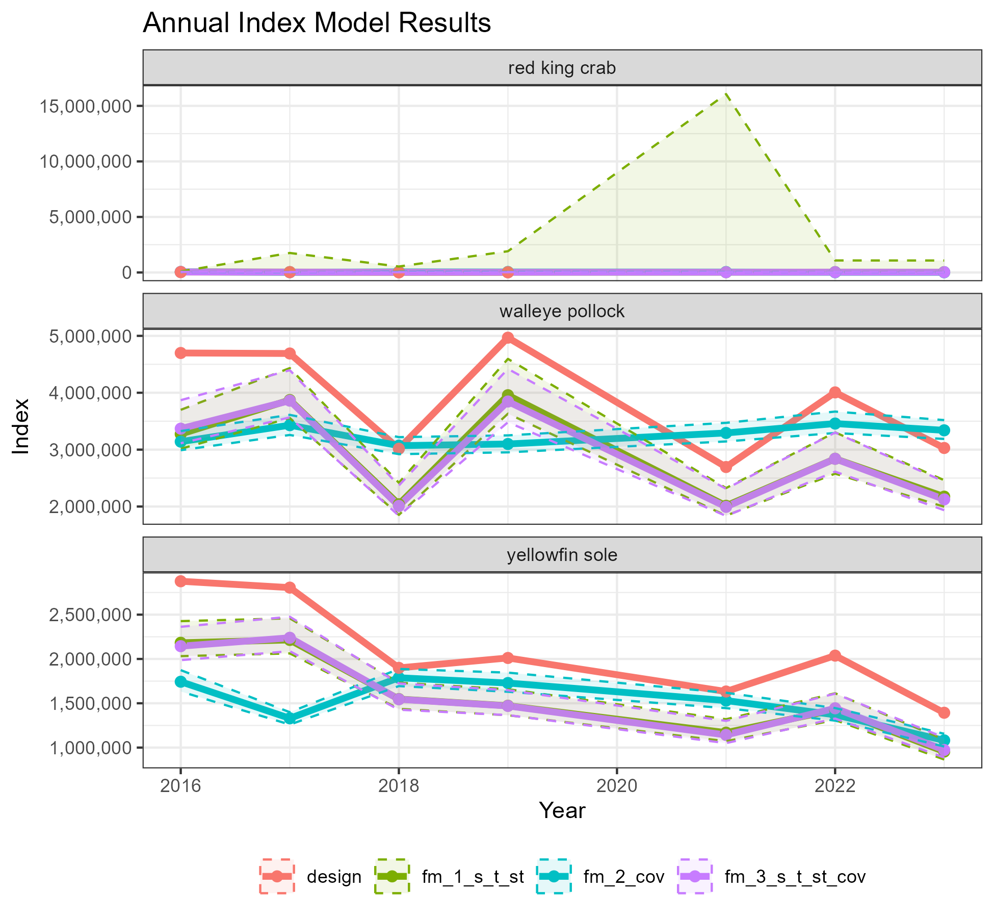
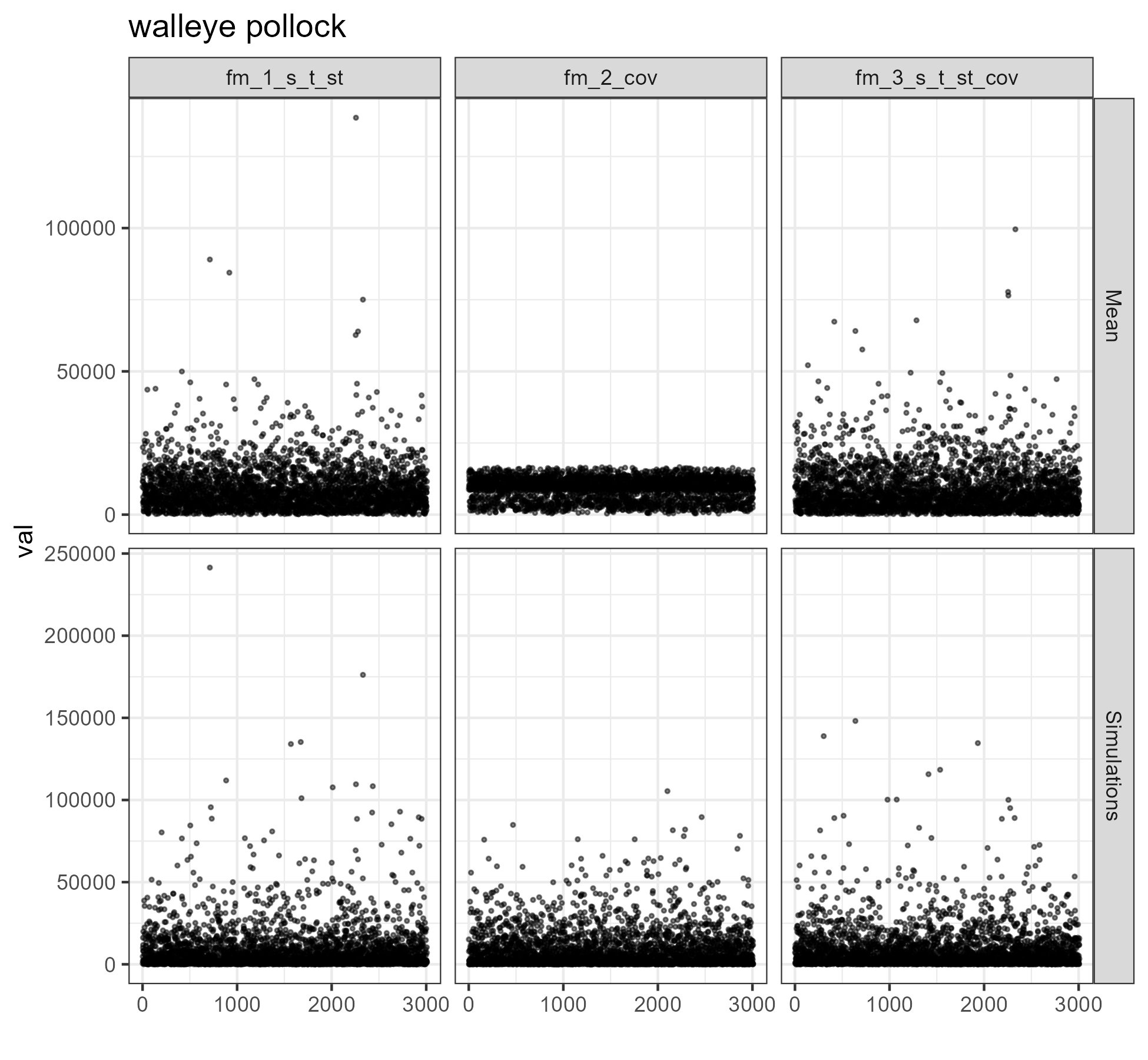
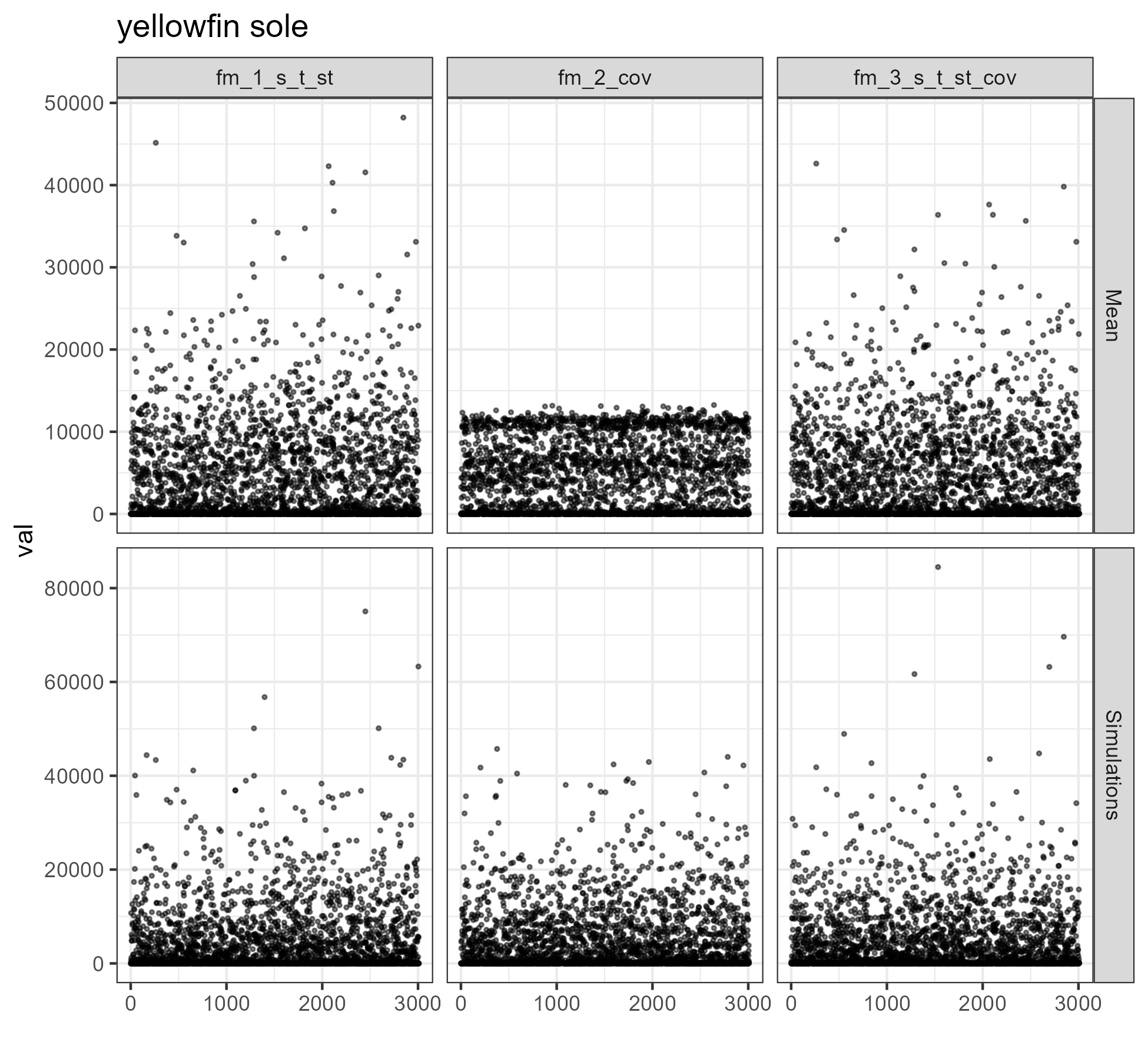
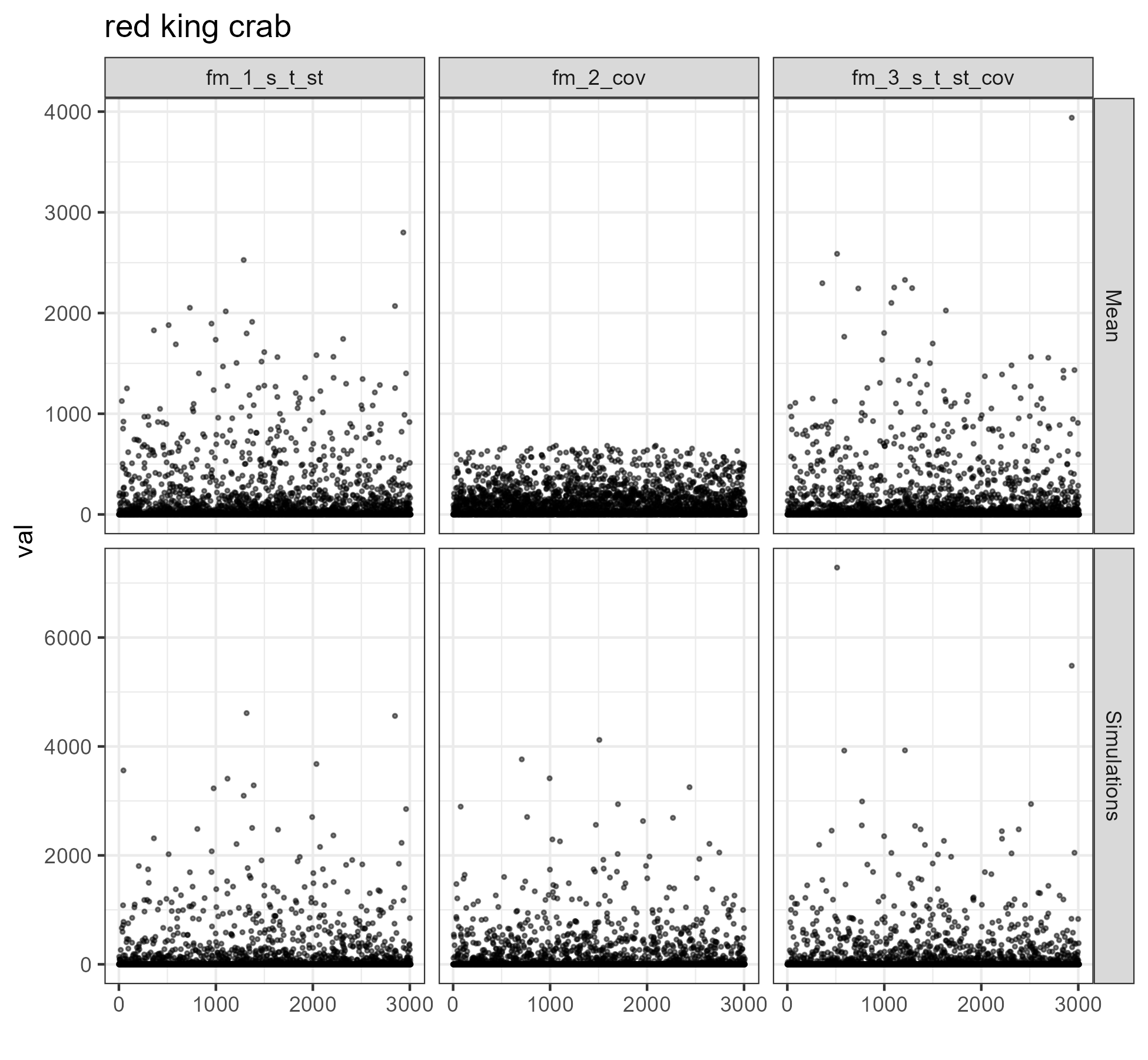
10. Simulations
sims <- fittimes <- list()

for(i in 1:nrow(comb)){
  cat("Simulating ",comb$SPECIES[i],"\n", comb$fm_name[i], ": ", comb$fm[i], "\n")

  temp <- paste0(comb$SPECIES[i], " ", comb$fm_name[i])

  fittimes[[ temp ]] <-
    system.time ( sims[[ temp ]] <-
                    sdmgamindex::get_surveyidx_sim(
                      model = models[[i]],
                      d = ds[[ comb$SPECIES[i] ]]) )

  sim <- sims[[ temp ]]
  fittime <- fittimes[[ temp ]]

  save(sim, fittime, file = here::here("inst",paste0("vigD_model_sims_",comb$SPECIES[i], "_", comb$fm_name[i],".Rdata")))
}
#>
#> red king crab fm_1_s_t_st: 5.3 minutes
#> red king crab fm_2_cov: 0.03 minutes
#> red king crab fm_3_s_t_st_cov: 6.2 minutes
#> walleye pollock fm_1_s_t_st: 5.3 minutes
#> walleye pollock fm_2_cov: 0.11 minutes
#> walleye pollock fm_3_s_t_st_cov: 5.4 minutes
#> yellowfin sole fm_1_s_t_st: 5.4 minutes
#> yellowfin sole fm_2_cov: 0.04 minutes
#> yellowfin sole fm_3_s_t_st_cov: 5.2 minutes
# par(mfrow = c(2, 2)) # Create a 2 x 2 plotting matrix
# for(i in 1:nrow(comb)){
# # png('output/my_plot.png')
#   plot(sims[[i]]$sim, main = paste0(names(sims)[i], " sims"))
#   plot(sims[[i]]$mu[[1]], main = paste0(names(sims)[i], " mu"))
# # dev.off()
# }

dat <- c()
for(i in 1:nrow(comb)){
    dat <- dat %>%
      dplyr::bind_rows(
        data.frame(
        SPECIES = comb$SPECIES[i],
        model = comb$fm_name[i],
        Simulations = as.vector(sims[[i]]$sim),
        Mean = as.vector(sims[[i]]$mu[[1]]),
        Index = 1:nrow(sims[[i]]$sim)) )
}

dat <- dat %>%
  tidyr::pivot_longer(cols = c("Simulations", "Mean"), names_to = "type", values_to = "val")

for (i in 1:length(unique(comb$SPECIES))) {
  figure <- ggplot2::ggplot(data = dat %>%
                              dplyr::filter(SPECIES == unique(comb$SPECIES)[i]),
                            mapping = aes(x = Index, y = val)) +
    ggplot2::geom_point(size = .5, alpha = .5) +
    ggplot2::facet_grid(rows = vars(type), cols = vars(model), scales = "free_y") +
    ggplot2::ggtitle(unique(comb$SPECIES)[i]) +
    ggplot2::xlab("")

ggsave(filename = paste0("vigD_model_sim_", unique(comb$SPECIES)[i], ".png"),
         path = here::here("vignettes"),
         plot = figure,
         width = 6.5, height = 6)
}
REPS <- 4
ests <- list()

for(i in 1:nrow(comb)){

  cat("Simulating ",comb$SPECIES[i],"\n", comb$fm_name[i], ": ", comb$fm[i], "\n")
  temp <- paste0(comb$SPECIES[i], " ", comb$fm_name[i])

  # for(SPECIES in specLevels){
  ests[[ temp ]] <- list()

  ## simulate data
  csim <- sdmgamindex::get_surveyidx_sim(models[[i]], ds[[comb$SPECIES[i]]])
  sims <-lapply(1:REPS,function(j) sdmgamindex::get_surveyidx_sim(
    model = models[[i]],
    d = ds[[comb$SPECIES[i]]],
    sampleFit = FALSE,
    condSim = csim) )

  ## re-estimate
  tmp <- ds[[i]]
  for(ii in 1:REPS) {
    tmp[[2]]$Nage <- matrix(sims[[ii]][[1]][,1],ncol=1)
    colnames(tmp$Nage)<-1

    ests[[SPECIES]][[ii]]  <-
      sdmgamindex::get_surveyidx(
        x = tmp,
        ages = 1,
        myids=NULL,
        predD=allpd,
        cutOff=0,
        fam="Tweedie",
        modelP=fm,
        gamma=1,
        control=list(trace=TRUE,maxit=10))
  }
}

sims
ests

png(filename = here::here("vignettes","vigD_model_simsest_plot.png"),
    width=640*pngscal,
    height=480)
# par(mfrow=c(2,2))
save(sims, ests, file = here::here("inst","vigD_model_simsest.Rdata"))
for(i in 1:nrow(comb)){
  sdmgamindex::plot_simulation_list(
    x = ests[[temp]],
    base=models[[temp]],
    main=temp,
    lwd=2)
}
dev.off()