September 2026 Assessment developments
Eastern Bering Sea walleye pollock

Artificial intelligence (AI) tools were used to aid document development and model implementation. AI-assisted material was reviewed and revised by the authors, who retain responsibility for the scientific content, code, analyses, interpretations, and conclusions.
Ianelli, James, Sophia Wassermann, Carey McGilliard, Grant Adams, Matt Cheng, Cody Szuwalski, and Cole Monnahan. 2026. September 2026 Assessment Developments: Eastern Bering Sea Walleye Pollock. Seattle, WA: Alaska Fisheries Science Center, National Marine Fisheries Service. https://noaa-afsc.github.io/EBS_pollock/doc/EBSpollock_Sept_2026.html.
1 Summary
Model 26.0 should be adopted as the operational model for calculating ABC and OFL and determining eastern Bering Sea pollock stock status for the November 2026 Bering Sea and Aleutian Islands Groundfish Plan Team review and the December 2026 Scientific and Statistical Committee (SSC) and Council considerations. The fall assessment should apply Model 26.0 to the completed 2025 fishery and 2026 survey updates and carry its fitted state into the standard Tier 3 projection workflow. This recommendation is supported by the Model 23.2 translation check, close agreement of population trajectories, successful convergence and simulated-data recovery, one-step-ahead residual checks, multi-start testing, lag-preserving retrospectives, survey-index sensitivities, and the reproducible spmR projection handoff. Model 23.0 provides the continuity benchmark for the review of this transition.
This working paper brings together eastern Bering Sea pollock assessment work that resumed after the 2025 funding lapse and federal furlough. It establishes a common review record for data preparation, model numbering, software translations, diagnostics, projections, and responses to Scientific and Statistical Committee (SSC) comments. The comparisons use the 1964–2024 data basis inherited from accepted Model 23.0. New 2025 and 2026 observations will enter the assessment after the source products, sample sizes, ageing-error treatment, and quality-control checks are complete.
The model numbering plan separates scientific purpose from software. Model 23.0 is the accepted 2024 ADMB assessment model. Model 23.1 is the direct RTMB translation check, and Model 23.2 is the Rceattle translation check. Model 25.0 is the RTMB development line begun in 2025, and Model 26.0 is the Rceattle development line begun in 2026. SPoRC provides a supporting comparison across the development lines. The Data section also separates two age-data questions: use of FT-NIRS predicted ages and revision of the method used to expand BTS age samples into annual proportions at age.
Model 25.0 reproduces the corrected full-age BTS ADMB bridge and supports continued evaluation of composition fit, selectivity, and retrospective stability. From 1978 through 2024, the matched Model 23.0 and Model 23.2 ADMB runs have correlations of 0.994 for spawning biomass and 0.999 for age-1 recruitment; their 2024 differences are +1.12% and -9.19%, respectively. The simple Model 26.0 Rceattle fit met the stated convergence criteria and closely followed the Model 23.2 Rceattle-aligned ADMB bridge, with trajectory correlations above 0.998. The ATS age-composition likelihood uses ages 2–15 and 18 fitted survey years; its 2020 row has sample size zero because no age-composition sample was collected. Composition residuals varied less than expected under the fitted model. Forty-seven of 50 dispersed-start fits returned to the best solution, while three reached the same higher objective. The repeated higher objective indicates a recurring alternative solution. All 50 simulated-data self-tests completed with convergence status OK. The lag-preserving nine-peel retrospective produced Mohn’s rho values of 0.331 for spawning biomass, 0.214 for total biomass, 0.188 for age-1 recruitment, and -0.127 for fishing mortality. The peels generally estimated greater biomass and recruitment and lower fishing mortality than the full fit over the same years. Controlled data tests for the 2020-to-2021 peel transition identified the 2021 BTS biomass index as the strongest single influence on spawning biomass, with the 2020 fishery age composition and 2021 BTS age composition also contributing to the revision. These results make composition fit, the recurring alternative solution, and retrospective stability the principal Model 26.0 evaluation priorities.
The whole-index-fleet sensitivities retained CPUE and removed BTS, ATS, or AVO in separate refits. All three completed with convergence status OK and positive-definite Hessians. BTS had the greatest influence: its removal reduced 2024 spawning biomass by 11.8% and increased 2024 fishing mortality by 96.9%. Removing ATS increased 2024 spawning biomass by 11.4% and age-1 recruitment by 34.5%. Removing AVO changed each 2024 quantity by less than 7%. These severe deletion tests show the complementary roles of the survey series and identify BTS as the principal source of scale information.
The spmR projections demonstrate a reproducible handoff from Model 26.0 to the standard seven-alternative projection workflow. Updated 2025 and 2026 data will provide the basis for ABC, OFL, and status determinations during the November and December 2026 review cycle. The exploratory recruitment analysis favored the model containing age-0 late-summer sea-surface temperature; its negative fitted pathway provides a testable in-sample association for further biological and predictive evaluation. The bridge, convergence tests, diagnostics, retrospective evaluation, index sensitivities, and projection handoff support the recommendation that Model 26.0 be adopted for 2026 management advice through the updated-data run and formal Plan Team, SSC, and Council review. Appendix 1 preserves the SSC comments and response plan, Appendix 2 provides the development framework for an Ecosystem and Socioeconomic Profile, Appendix 3 evaluates time- and age-varying BTS availability, and Appendices 4–7 document the exploratory SparseNUTS run, reproducible model workflow, observation continuity and case-deletion influence, and acronym glossary. Appendix 8 documents fishery length-frequency patterns.
2 Introduction
This document brings together eastern Bering Sea pollock assessment work affected by the 2025 funding lapse and federal furlough. Routine SAFE preparation, review, and archiving paused during that period. After work resumed, data preparation and model development progressed on different schedules. This report restores a single review record for the data updates, model numbering, ADMB-to-RTMB bridge, and 2026 RTMB and Rceattle development.
The main report is organized around the decisions needed for the 2026 review. The Model specifications section defines the model numbers and their roles so results can be traced to the correct scientific configuration. The Data section summarizes the shared assessment inputs and identifies age-data issues that need consistent treatment across platforms. The Model results section presents the translation checks, Model 26.0 fit and diagnostics, retrospective evaluation, sensitivities, projections, and exploratory recruitment pathways needed to judge readiness for assessment use. The Conclusion brings that evidence together and states the recommended role and next steps for Model 26.0 during the November and December review cycle.
The appendices preserve supporting material that informs this work. Appendix 1 presents the main SSC comments and planned responses and retains the earlier 2024 comments. Appendix 2 provides the development structure for an EBS pollock Ecosystem and Socioeconomic Profile (ESP). Appendix 3 evaluates time- and age-varying BTS availability, Appendix 4 reports exploratory SparseNUTS sampling, Appendix 5 records the reproducible model workflow, Appendix 6 evaluates observation continuity and case-deletion influence, and Appendix 7 defines the report’s acronyms. Appendix 8 summarizes seasonal and spatial patterns in the observed pollock length-frequency samples. Together, the main sections and appendices connect the resumed work with the assessment review record.
3 Model specifications
3.1 Model numbering plan
The model number should identify the model’s place in the review record. The software name should be shown separately. Under this plan, Model 23.0 is the 2024 ADMB source, Model 23.1 is its direct RTMB translation check, and Model 23.2 is the Rceattle translation check. The newer model names are Model 25.0 (RTMB) for the work begun in 2025 and Model 26.0 (Rceattle) for the development line begun in 2026. The flowchart shows the two numbered development lines and SPoRC’s supporting comparison role (Figure 1).
flowchart LR accTitle: EBS pollock assessment model numbering and development history accDescr: Flowchart from the 2024 Model 23.0 ADMB source through the Model 23.1 RTMB translation check to the Model 25.0 RTMB line, and through the Model 23.2 Rceattle translation check to the Model 26.0 Rceattle line, with SPoRC supporting comparisons of the two development lines. A["Model 23.0<br/>2024 ADMB source"] -->|"direct translation<br/>and checks"| B["Model 23.1<br/>RTMB translation check"] B --> C["Model 25.0<br/>RTMB line begun in 2025"] A -->|"Rceattle bridge<br/>and checks"| E["Model 23.2<br/>Rceattle translation check"] E --> D["Model 26.0<br/>Rceattle line begun in 2026"] S["SPoRC<br/>supporting comparison"] -.->|"common tests"| C S -.->|"common tests"| D classDef model fill:#e8f0f7,stroke:#52616b,color:#111111 classDef comparison fill:#fff4cc,stroke:#9a8444,color:#111111 class A,B,C,D,E model class S comparison
The labels should be used as follows:
- Model 23.0 (ADMB) identifies the accepted source model used in 2024.
- Model 23.1 (RTMB) identifies the direct translation used to check that the new code reproduces Model 23.0. Its role is a numbered translation check, while Model 23.0 continues to support management advice.
- Model 23.2 (Rceattle) identifies the Rceattle translation check aligned with the modified ADMB bridge. It provides the direct reference for Model 26.0 implementation checks.
- Model 25.0 (RTMB) is the public name for the RTMB assessment line begun in 2025 at the SSC’s request.
- Model 26.0 (Rceattle) is the public name for the Rceattle development line begun in 2026. List its scientific changes separately from the software change. Its bridge, diagnostics, retrospective behavior, and projections support the recommendation for its 2026 operational role. Model 23.0 provides continuity through the formal review transition.
- SPoRC remains a supporting comparison. The single-region EBS pollock vignette illustrates the bridge from Model 23.0 to SPoRC and identifies the current differences between the implementations. Research on pollock movement and connections between U.S. and Russian waters is progressing. A numbered model name would apply when SPoRC advances as an assessment candidate.
For later variants, keep the main number and add a decimal suffix, such as 26.1 or 26.2. Each suffix should represent one clearly documented change. Use the same label in the report, tables, presentations, run folders, and archive.
4 Data
4.1 Data summary
The current cross-platform comparison uses the sex-combined, ages 1–15 data basis inherited from the 2024 Model 23.0 assessment. The population time series extends from 1964 through 2024. Fishery age compositions extend through 2023 because of the normal processing lag. The same underlying assessment observations are translated into the ADMB, RTMB, SPoRC, and Rceattle input structures. Each model retains its own fit calculations, sample-size conventions, and data organization. The accepted assessment and 2024 model-evaluation documents provide the overall data lineage (Ianelli et al. 2023; Ianelli and McGilliard 2024).
The basic data used across the platforms are:
- Fishery data: annual retained catch from 1964 through 2024, fishery age compositions from 1964 through 2023, empirical fishery weight at age, and the historical fishery catch-per-unit-effort (CPUE) index for 1965–1976.
- Bottom-trawl survey (BTS): the biomass index and its covariance, age compositions, sample sizes, and survey weight at age for 42 survey years during 1982–2024. The standard survey was absent in 2020. Model-based estimation of pollock survey indices and age compositions is described by O’Leary et al. (2020), and spatially structured estimation of pollock weight at age is described by Indivero et al. (2023).
- Acoustic-trawl survey (ATS): pollock abundance indices and weight at age for 19 survey years during 1994–2024, with age compositions and sample sizes for 18 of those years. No age-composition sample was collected in 2020. The survey series includes separate information for age-1 pollock and older pollock. Survey methods are documented by Honkalehto and McCarthy (2015); current work on uncertainty in acoustic-trawl estimates is described by Urmy et al. (2025).
- Supplementary abundance indices: the acoustic vessel-of-opportunity (AVO) series has 18 observations during 2006–2024, and the historical CPUE series has 12 observations during 1965–1976. The AVO approach and recent reanalysis are described by Honkalehto et al. (2011) and Lauffenburger et al. (2024).
- Biological schedules: the models use ageing-error information, maturity, natural mortality, and spawning, fishery, and survey weight-at-age schedules. AFSC pollock ageing methods and data quality are summarized by Matta et al. (2026); spatial and temporal variation in EBS pollock weight at age is evaluated by Indivero et al. (2023).
Across platforms, ADMB Model 23.0 provides the accepted 2024 assessment reference, observation schedule, and source-model settings. RTMB Models 23.1 and 25.0 use the corrected ADMB bridge inputs directly and preserve the complete ages 1–15 BTS composition treatment.
The summary above describes the common 2024-terminal bridge used for model comparison. New 2025 and 2026 observations will enter the assessment only after their source products, sample sizes, ageing-error treatment, and quality control have been finalized.
4.2 Issues
This section documents two distinct age-composition product issues considered after the 2024 assessment: the method used to assign ages to individual otoliths and the spatio-temporal method used to expand BTS age samples into annual proportions at age. The first concerns traditional microscope ages (TMA) versus ages predicted by Fourier-transform near-infrared spectroscopy (FT-NIRS). The second concerns replacement of the prior BTS age-composition estimator with a tinyVAST implementation. In the second case, the survey observations remain the same; the estimated annual age-composition data product derived from those observations has changed because the expansion method was revised. These changes occur at different stages of the data workflow and should be evaluated separately.
4.2.1 FTNIRS age-data
The Alaska Fisheries Science Center’s Age and Growth Program has produced more than 460,000 walleye pollock age estimates since 1971. From 2005 through 2024, annual production averaged 11,141 pollock ages and ranged from 8,408 to 14,441. Across Alaska pollock stocks, inter-reader precision was relatively high: the overall average coefficient of variation was 4.28%, percent agreement was 68.6%, and reader and tester estimates generally differed by one year or less year. Eighty percent of pollock aged by the program were 3–10 years old, and the maximum observed age was 31 years. Radiometric analysis supports the accuracy of the program’s ageing criteria through age 8, while marginal increment analyses, year-class tracking, hard-structure comparisons, and captive-rearing studies provide additional corroboration. Older ages occur more frequently in the Bering Sea and Aleutian Islands than in the Gulf of Alaska, and Bering Sea pollock generally grow more slowly but attain greater lengths and ages. Female pollock also become larger at age than males beginning at approximately age 5 (Matta et al. 2026, 33–42). These production and precision statistics summarize AFSC pollock ageing across Alaska stocks rather than the eastern Bering Sea alone; the eastern Bering Sea assessment is the most data-rich pollock assessment.
These results describe traditional microscope ageing (TMA), which assigns age by preparing an otolith and visually counting annual growth zones. FT-NIRS is being developed as a rapid secondary ageing method that depends on reference ages produced through traditional microscopic examination (Matta et al. 2026). FT-NIRS measures the wavelengths and amount of near-infrared light absorbed by an otolith and predicts age from its spectral and chemical signal using a calibration model. It can process otoliths substantially faster, but its predicted ages are methodologically different from direct microscope readings (NOAA Fisheries age-method overview). The established scale, precision, and corroboration of the TMA series therefore provide important context for evaluating whether FT-NIRS predictions preserve the age structure and cohort signals used by the assessment.
The 2025 CIE discussion paper compared the two methods using pollock data. For the same design-based BTS abundance-at-age inputs, TMA estimates showed a high degree of cohort consistency, whereas FT-NIRS estimates showed lower cohort consistency; the assessment authors described the consequence of that difference as unresolved. The comparison also identified differences between TMA- and FT-NIRS-based proportions at age for the fishery, BTS, and ATS. Model tests therefore treated FT-NIRS ages as a separate data source and considered both global and fleet-specific FT-NIRS age-error matrices. See the official FT-NIRS data consistency comparisons for the cohort plots, composition comparisons, data coverage, and alternative age-error treatments.
The FT-NIRS issue concerns age assignment and associated ageing error. The BTS bridge below concerns the subsequent expansion of age observations across space and time. Its scope is the expansion method; a separate analysis compares TMA with FT-NIRS.
4.2.2 Impact of revised BTS age-composition estimates
This section isolates the effect of replacing the original bottom-trawl survey (BTS) estimates of proportions at age in BTSProp.csv with the revised estimates in tinyVAST_props_new.csv. The age-composition data product changes while the underlying survey data remain the same. Both ADMB runs use the complete 2025 input set and the same model specification, executable, starting parameter file, and tinyVAST 2025 BTS age-composition estimate. The sensitivity restores the original 1982-2024 BTS proportion estimates while holding the 2025 tinyVAST row constant. The comparison therefore addresses the historical estimator change.
The 2024 assessment used the previous spatio-temporal expansion of BTS age samples. The revised series uses an improved implementation in tinyVAST, a multivariate spatio-temporal generalized linear mixed-model framework that can model age groups jointly, share information across locations and years, and area-expand predictions to annual abundance and proportions at age (Thorson and Haltuch 2019; Thorson et al. 2025). The tinyVAST age-composition expansion example documents this workflow for EBS pollock age data. This methodological update changes the estimated BTS proportions at age supplied to the assessment; the controlled runs below quantify the resulting assessment-model effect while holding the other inputs and model configuration fixed.
The controlled input comparison changes the historical BTS age-composition product while holding the 2025 age composition and every other assessment input constant (Table 1).
| BTS Age-Data Contrast | |
| metric | value |
|---|---|
| Historical BTS years replaced | 42 |
| First replaced year | 1982 |
| Last replaced year | 2024 |
| 2025 BTS age row held constant | Yes |
| Maximum absolute proportion-at-age difference | 0.015778407 |
The derived-product comparison uses the both region from BTSProp.csv as the original estimated series and tinyVAST_props_new.csv as the revised estimated series (Figure 2). Across the 42 matched survey years, relative changes range from -11.9% to +54.8%; the largest absolute change is 1.58 percentage points. The calculation uses the original estimated proportion as the denominator and describes the revision to the derived age-composition product rather than a change in the survey observations or its influence on model results. The revised 2025 row is excluded because the original file ends in 2024.
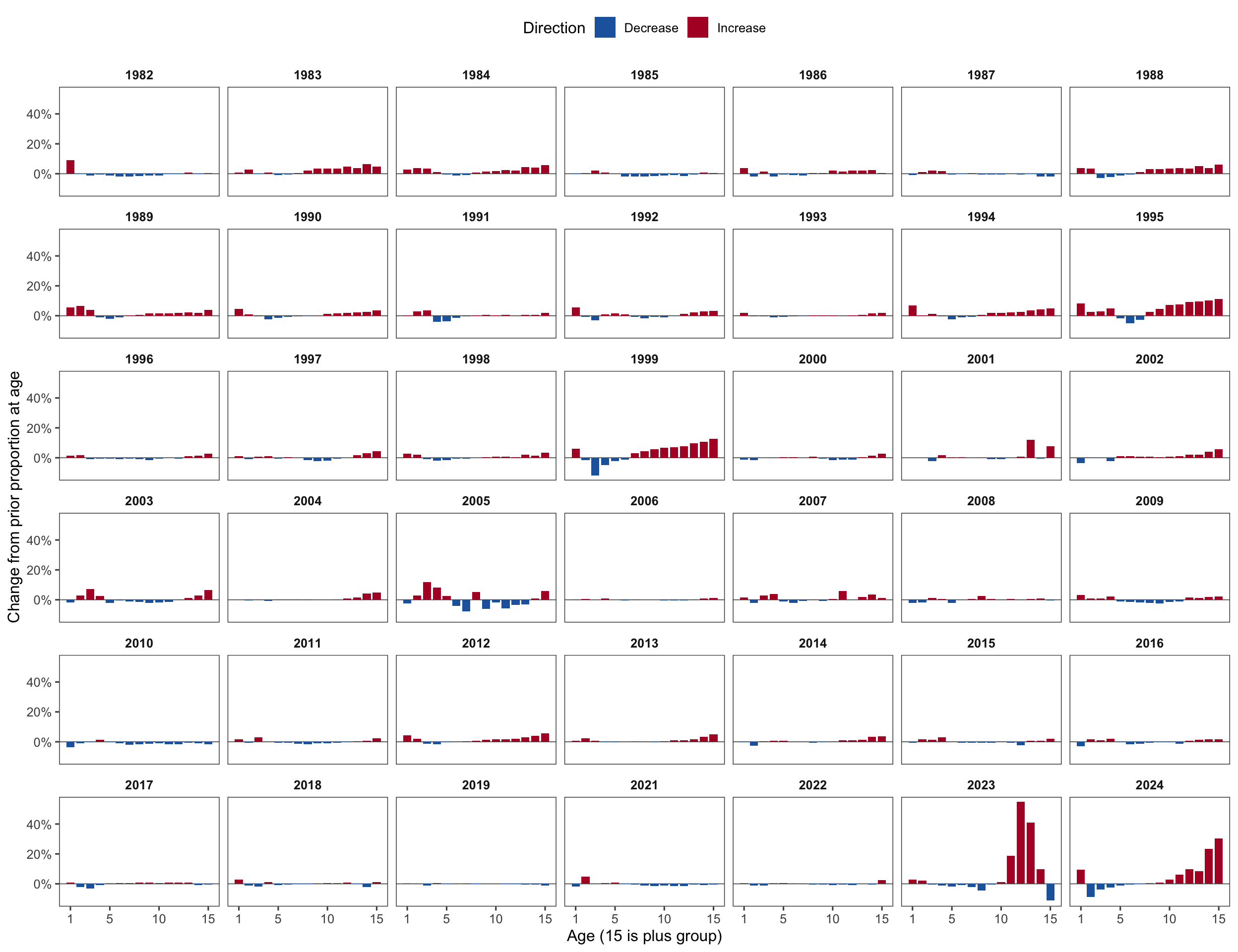
Both runs reached maximum absolute gradients below 0.001. The likelihood components in Table 2 document the fits and support a structured contrast between scenarios with different observed BTS age values.
| BTS Age-Data Bridge Diagnostics | ||||
| Data version | Total NLL | BTS index NLL | BTS age NLL | Maximum |gradient| |
|---|---|---|---|---|
| Current tinyVAST BTS ages | 7,062.470 | 32.673 | 211.608 | 4.97 × 10⁻⁴ |
| Prior BTSProp ages for 1982-2024 | 7,061.360 | 32.856 | 210.849 | 2.07 × 10⁻⁴ |
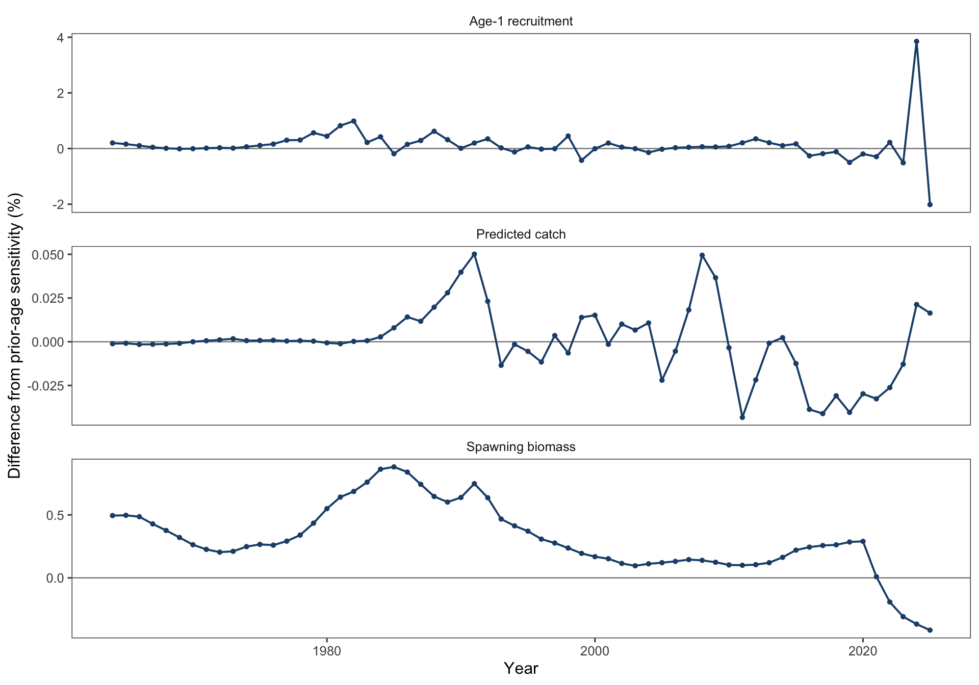
The revision changes terminal spawning biomass by -0.415%. The largest spawning-biomass difference is 0.881% in 1985. Terminal age-1 recruitment changes by -2.015%, which is the largest recruitment difference in the series. Terminal predicted catch changes by +0.016%. The terminal and maximum differences for each assessment quantity are summarized in Table 3.
| Effects of tinyVAST Historical BTS Proportions | ||||
| Quantity | Terminal year | Terminal difference (%) | Maximum absolute difference (%) | Year of maximum |
|---|---|---|---|---|
| Predicted catch | 2025 | 0.016 | 0.050 | 1991 |
| Age-1 recruitment | 2025 | −2.015 | 3.851 | 2024 |
| Spawning biomass | 2025 | −0.415 | 0.881 | 1985 |
Across years, spawning-biomass and predicted-catch differences remain small, while age-1 recruitment shows the larger year-to-year response (Figure 3).
4.2.3 Planned 2026 survey-data update
Data from the 2026 Acoustic-Trawl Survey (ATS), along with 2026 AVO data, will be added to this report after processing and quality-control review are complete. The update will identify any resulting changes to the relevant time series, figures, tables, and model inputs.
5 Model results
5.1 Model 23.1
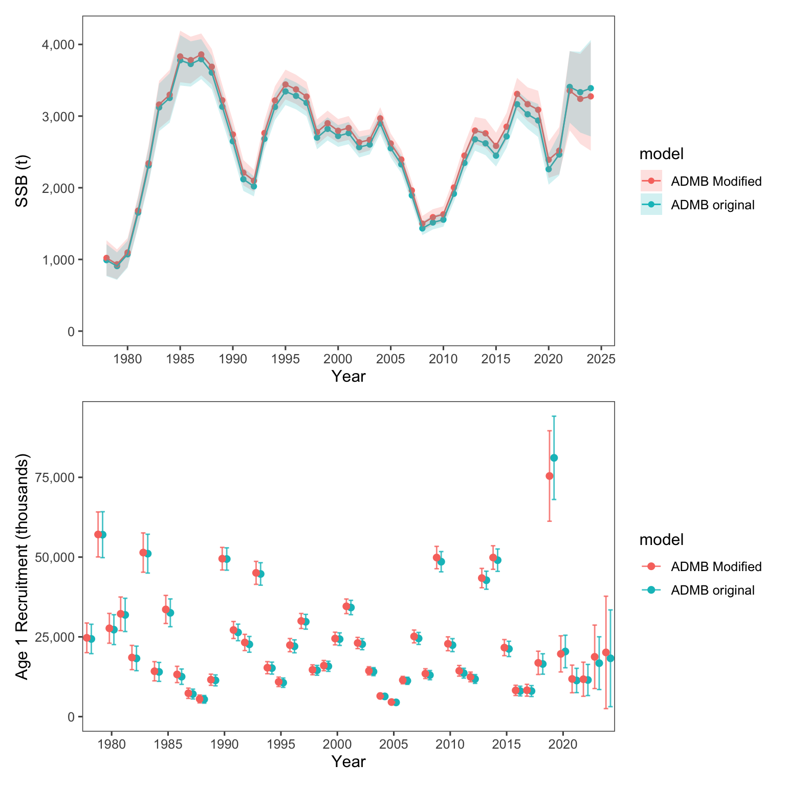
The September 2025 ADMB-to-RTMB bridge documented the small ADMB changes made before checking the direct RTMB translation. For the model numbering used here, ADMB original = Model 23.0 and ADMB Modified = Model 23.1. The second label identifies the adjusted ADMB version used to build and check Model 23.1 in RTMB. Model 23.1 serves as a translation check, while Model 23.0 continues to support management advice.
The spawning biomass and age-1 recruitment comparisons are reproduced in Figure 4. The source analysis attributes most of the small differences between the series to a revised rule for fishery selectivity, specifically the penalty applied when selectivity declines after age 6.
5.2 Model 25.0
The RTMB implementation matches the corrected ADMB bridge, including the full BTS age range, at the same best-fitting ADMB values, called maximum-likelihood estimates. Observed and predicted BTS age compositions each cover ages 1–15 and sum to one. Integer sample sizes set their influence in the multinomial likelihood, the fit calculation for age proportions. The total number of fish used to scale the age composition retains its ages 2–15 definition. The fitted BTS survey index measures biomass. Comparison with the historical configuration shows the effect of correcting the treatment of BTS data in the model fit.
The same corrected base model supports the one-step-ahead (OSA) checks, the analysis fitted only to BTS data (Only-BTS sensitivity), nine retrospective peels that remove recent years in sequence, and stock-production-model (SPM) projections. The retrospective procedure accounts for reporting lags among data streams and uses the previous year’s selectivity curve for the final year. Positive Mohn’s rho values, which summarize the direction and size of retrospective change, identify a stability concern for continued evaluation. Simulation testing and review will guide future operational refinements. Current management advice uses the accepted ADMB assessment model. The hierarchical Form-2 results generated with SparseNUTS describe a separate selectivity option.
5.3 Model 26.0
5.3.1 RCeattle implementation
Model 26.0 uses the common 1964–2024 bridge data described in Section 4.1. This run was fitted with Rceattle version 5.23.0 from the dsem-v5-integration branch, pinned at commit adf22f84b399e84e3b9a707e0b3bbb1624179a27. The version number and commit are reported together because the run represents a branch snapshot.
The simple configuration retains non-parametric selectivity for the fishery, acoustic vessel-of-opportunity (AVO), acoustic-trawl survey (ATS), and historical catch-per-unit-effort series. The bottom-trawl survey (BTS) retains the logistic curve and separate age-1 component used in the bridge. Annual selectivity changes follow the established random-walk configuration. The 2D age-by-year AR1 formulation remains a separate research sensitivity, allowing this analysis to focus on the simpler assessment structure requested for Model 26.0. The data-flow diagram shows how the shared observations support the fitted population states, bridge comparison, diagnostics, projections, and environmental-pathway analysis (Figure 5).
The Model 26.0 configuration retains ages 1–15, the established selectivity forms, and the two-stage fitting sequence (Table 4). The current branch retains the time-varying parametric BTS field as a compatibility setting and directs future development toward the newer selectivity-linkage interface. This run keeps the compatibility setting to match the bridge configuration. A later Model 26.x comparison can evaluate the interface change separately.
Both fitting stages met the current Rceattle convergence criteria. Model 26.0 had a maximum absolute gradient of \(4.98\times10^{-5}\), a positive-definite Hessian, and a Hessian condition number of 489,317. The weakest direction remains associated with the shared ATS/AVO annual selectivity changes (Table 5).
The analysis is archived as separate R scripts for the assessment fit and OSA checks, DSEM pathways, retrospective analysis, retrospective data sensitivity, whole-index-fleet sensitivity, spmR projections, and self-test.
flowchart TB
accTitle: Simple Model 26.0 data and analysis flow
accDescr: A top-to-bottom flowchart shows assessment inputs entering the simple Rceattle population model. Its fitted states support the bridge comparison, diagnostics, projection, and exploratory DSEM analyses.
subgraph I["Assessment inputs"]
direction TB
A["Catch and abundance indices"]
B["Ages 1-15 composition data"]
C["Maturity, mortality, weight,<br/>and ageing error"]
end
A --> M["Model 26.0<br/>Rceattle 5.23.0"]
B --> M
C --> M
M --> S["Abundance, recruitment,<br/>fishing mortality, selectivity"]
subgraph O["Model evaluation and use"]
direction TB
V["Model 23.2 bridge comparison"]
D["OSA, jitter, self-test,<br/>index sensitivity, retrospective"]
P["spmR projection"]
E["Exploratory DSEM pathways"]
end
S --> V
S --> D
S --> P
S --> E
classDef input fill:#e8f0f7,stroke:#52616b,color:#111111
class A,B,C,M,S,V,D,P,E input
| Item | Model 26.0 setting |
|---|---|
| Assessment years and ages | 1964–2024; ages 1–15 |
| Composition fit | MultinomialAFSC; likelihood sample sizes retained from the bridge workbook, with ATS 2020 set to zero |
| 2020 ATS age composition | Excluded from fitting because no age-composition sample was collected |
| Non-parametric selectivity | Fishery, AVO, ATS, and historical CPUE |
| BTS selectivity | Logistic curve with the separate age-1 component retained from the bridge |
| Time variation | Established random-walk selectivity changes |
| Natural mortality | Fixed age schedule used in the bridge |
| Fitting sequence | Scale fit with annual selectivity changes held constant, followed by the full simple fit |
| Fit | Objective | Maximum gradient | Positive-definite Hessian | Status |
|---|---|---|---|---|
| Stage 1 scale fit | 561.986 | 0.000162 | Yes | OK |
| Model 26.0 | 715.868 | 0.0000498 | Yes | OK |
5.3.2 Model 23.2 bridge comparison
For this comparison, Model 23.2 identifies the Rceattle-aligned ADMB bridge configuration. It contains the structural and likelihood changes needed to place the ADMB and Rceattle calculations on a common basis. Model 23.2 therefore provides the closest reference for evaluating the fitted Model 26.0 trajectories, while Model 23.1 continues to identify the direct RTMB translation described earlier.
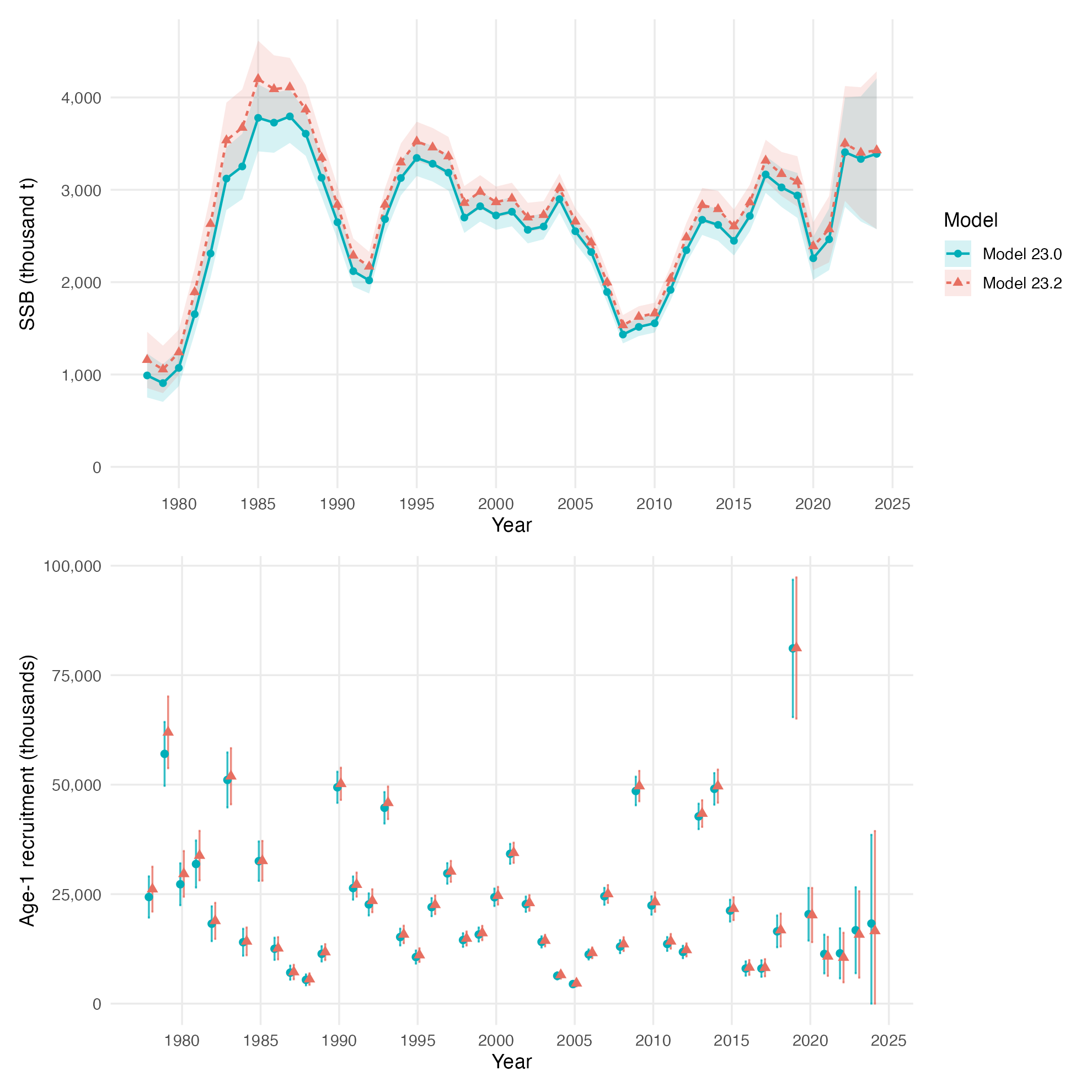
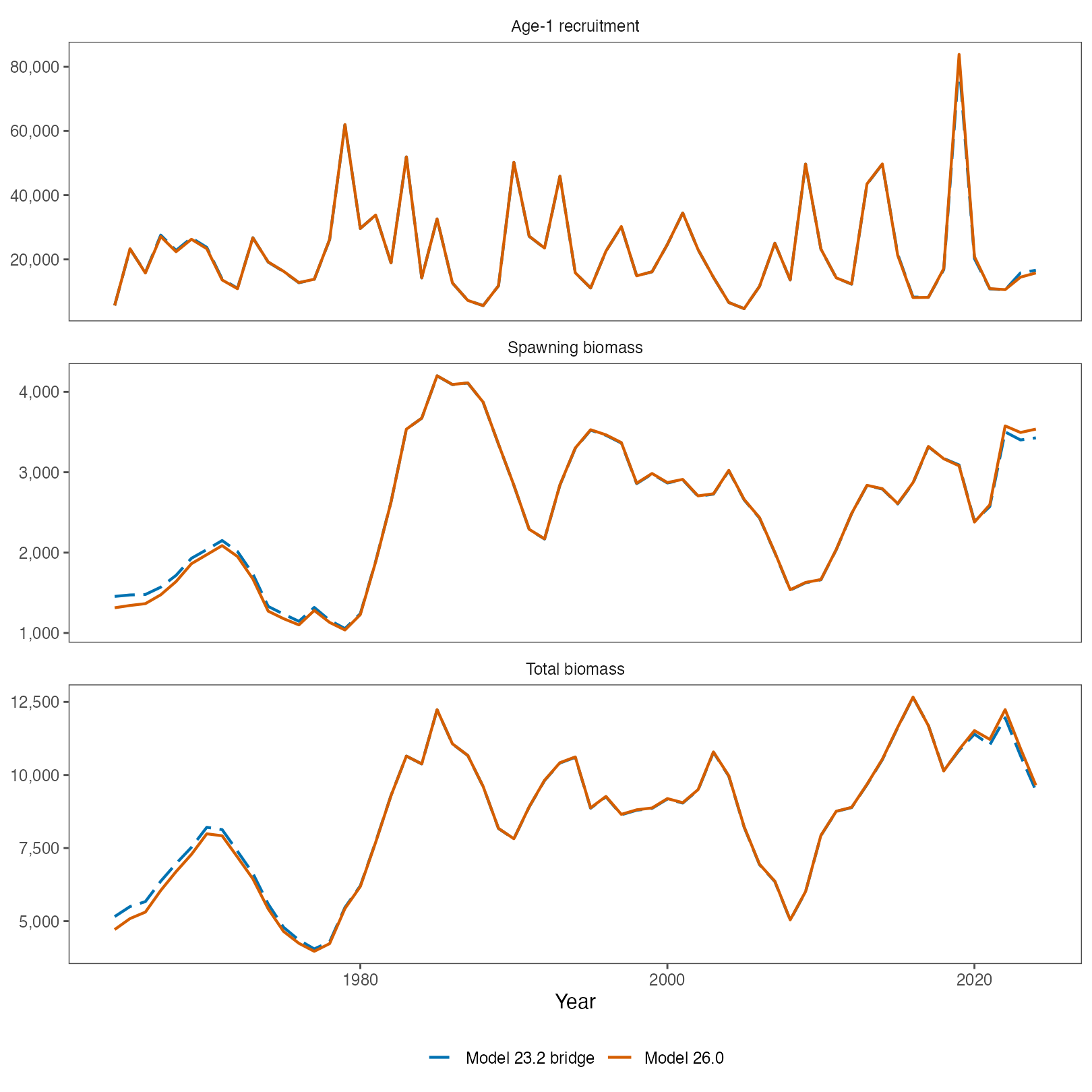
The matched Model 23.0 and Model 23.2 ADMB runs use the same input selector and shared data files. From 1978 through 2024, their spawning biomass trajectories have a correlation of 0.994 and a mean absolute difference of 7.15%. Their age-1 recruitment trajectories have a correlation of 0.999 and a mean absolute difference of 3.26%. In 2024, Model 23.2 spawning biomass is 1.12% higher and age-1 recruitment is 9.19% lower than Model 23.0. The uncertainty intervals overlap broadly across the displayed period (Figure 6).
The three Model 26.0 trajectories have correlations above 0.998 with the Model 23.2 bridge, and their mean absolute differences range from 0.72% to 1.46% (Table 6). The fitted trajectories closely follow the bridge over the full assessment period (Figure 7). The remaining differences reflect parameter estimation in Rceattle rather than a fixed-parameter translation test.
The annual comparison data, summary, and source record preserve the paired estimates, standard errors, run summaries, and file checksums used for the comparison.
| Quantity | Correlation | Mean absolute difference | 2024 difference |
|---|---|---|---|
| Spawning biomass | 0.9992 | 1.46% | +3.19% |
| Age-1 recruitment | 0.9997 | 0.72% | -5.05% |
| Total biomass | 0.9989 | 1.18% | +1.86% |
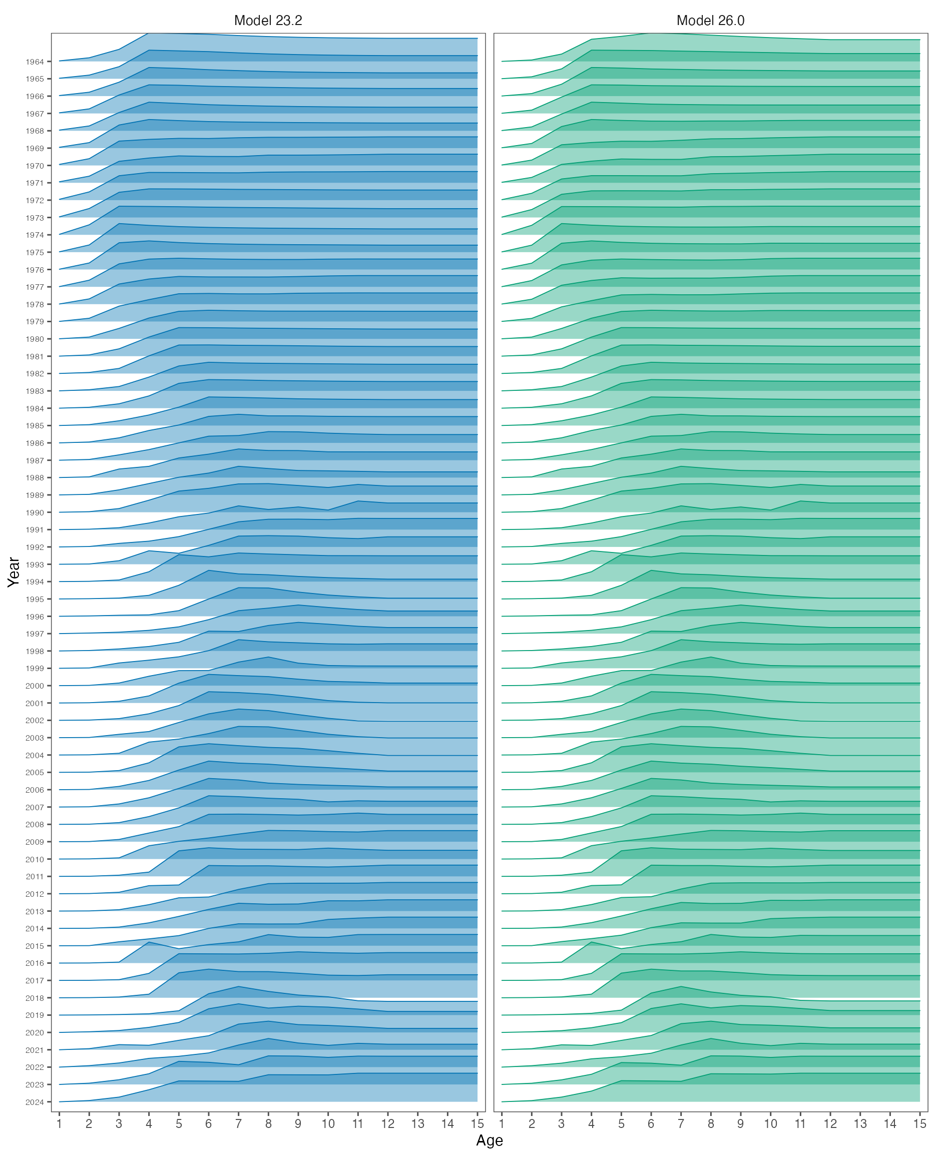
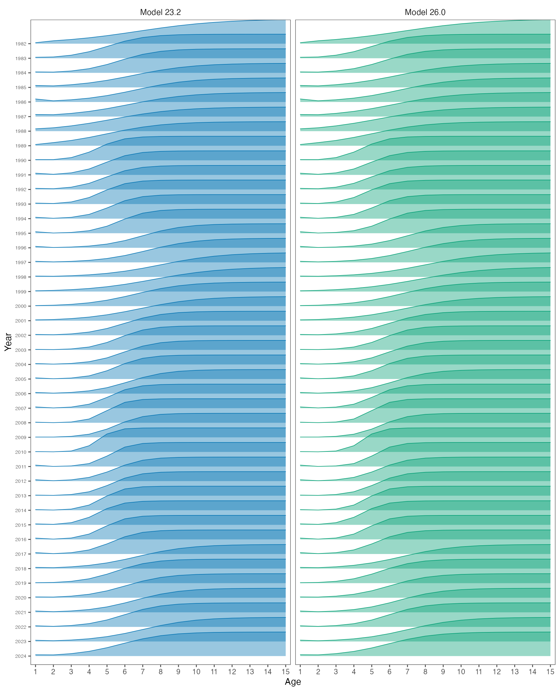
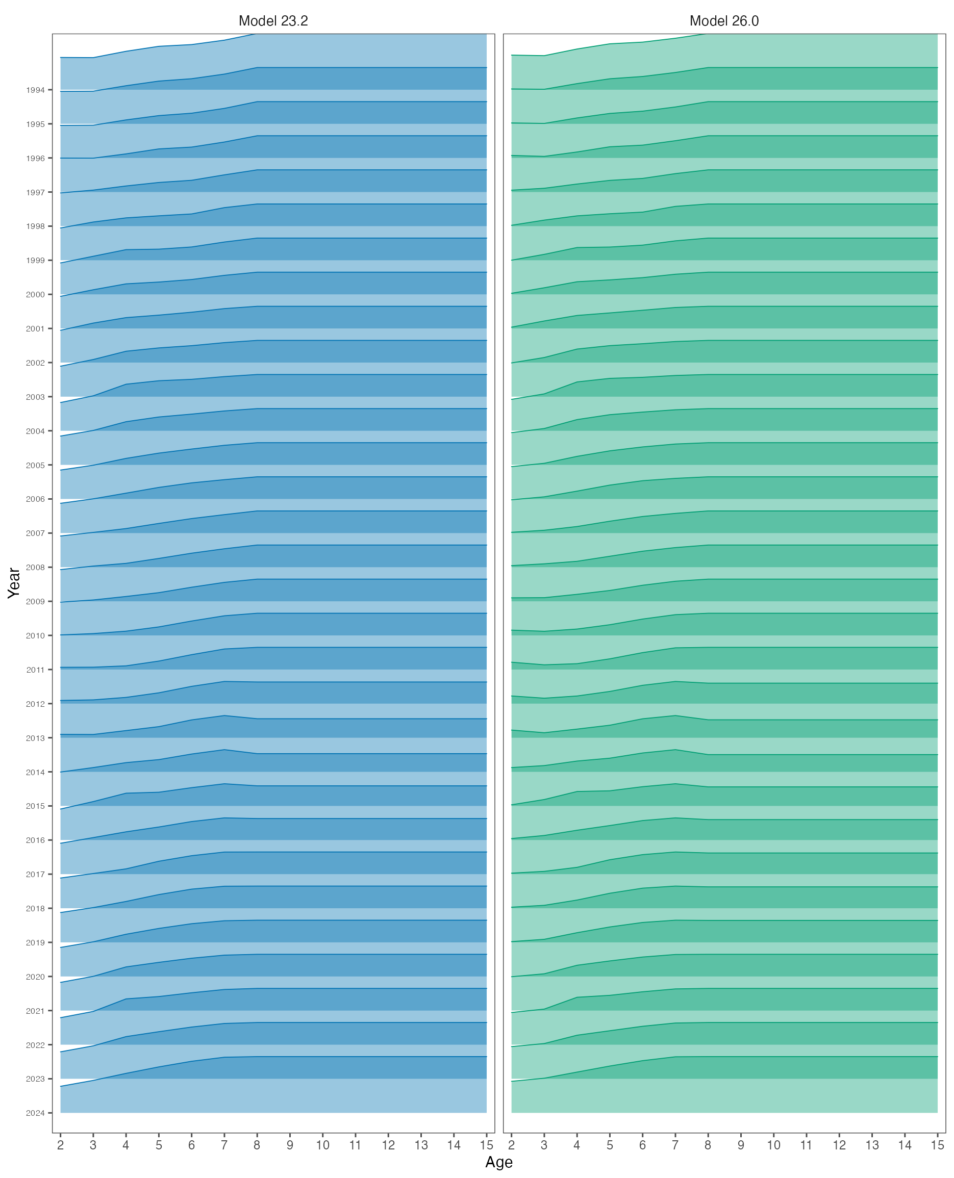
The annual selectivity comparisons place Model 23.2 on the left and Model 26.0 on the right. Each curve is divided by its annual maximum, so the figures compare shape rather than scale. Fishery curves cover 1964–2024, BTS curves cover 1982–2024, and ATS curves cover 1994–2024. Across the matched ages and years, the normalized curves have correlations of 0.997 for the fishery, greater than 0.999 for BTS, and 0.878 for ATS. The fishery and BTS shapes align closely, while the ATS comparison shows more age-specific differences (Figure 8–Figure 10). The selectivity comparison data retain the unscaled and normalized annual values.
5.3.3 Model fits
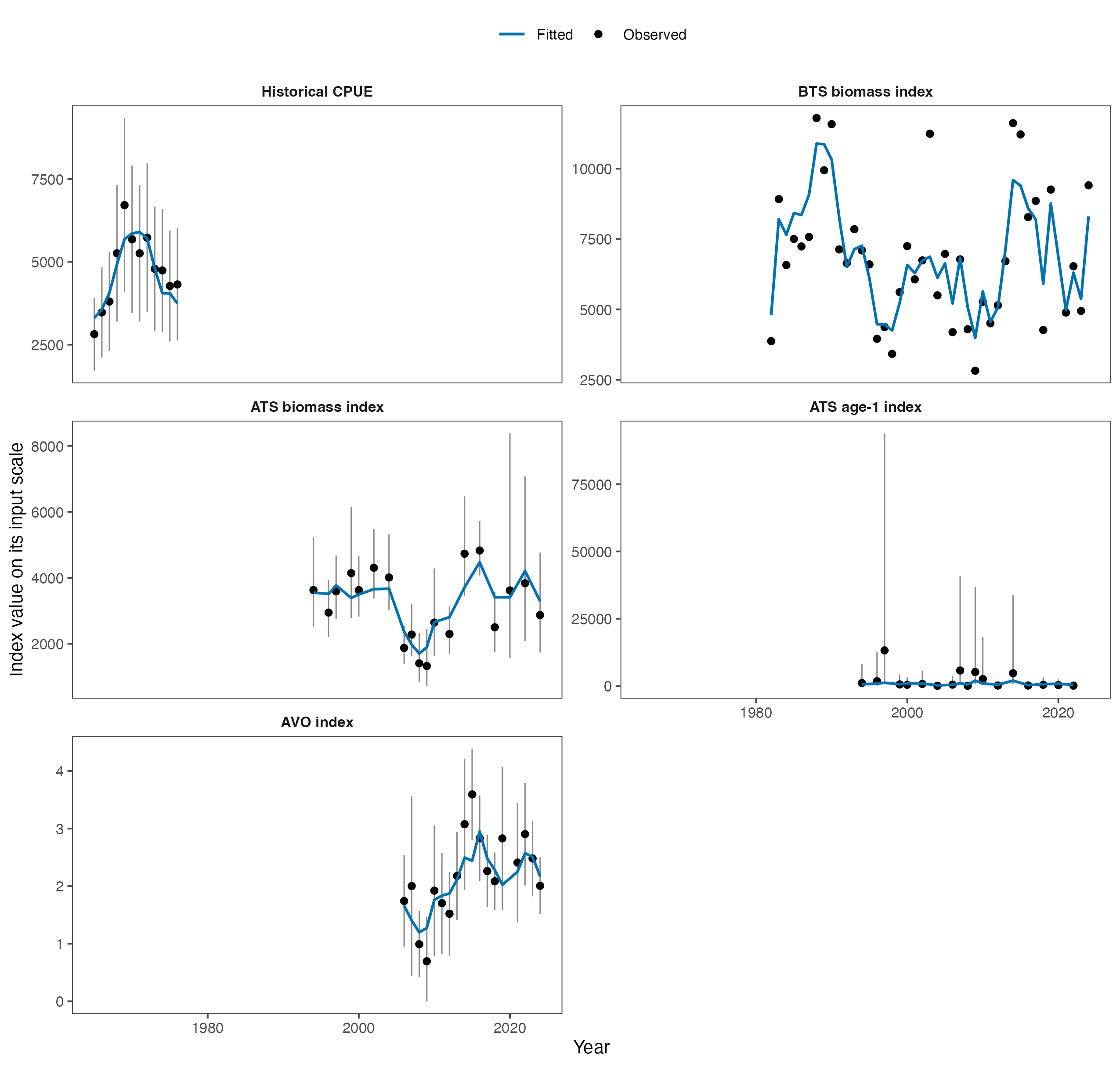
The fitted abundance indices generally follow the observed changes through time (Figure 11). Correlations between observed and fitted values are 0.90 for BTS, 0.88 for the ATS biomass index, 0.89 for the historical catch-per-unit-effort series, and 0.81 for AVO. The separate ATS age-1 index has a correlation of 0.60 and wider observation intervals in several years. Each panel retains the input scale for that series, so the vertical ranges are intended for comparison within a panel.
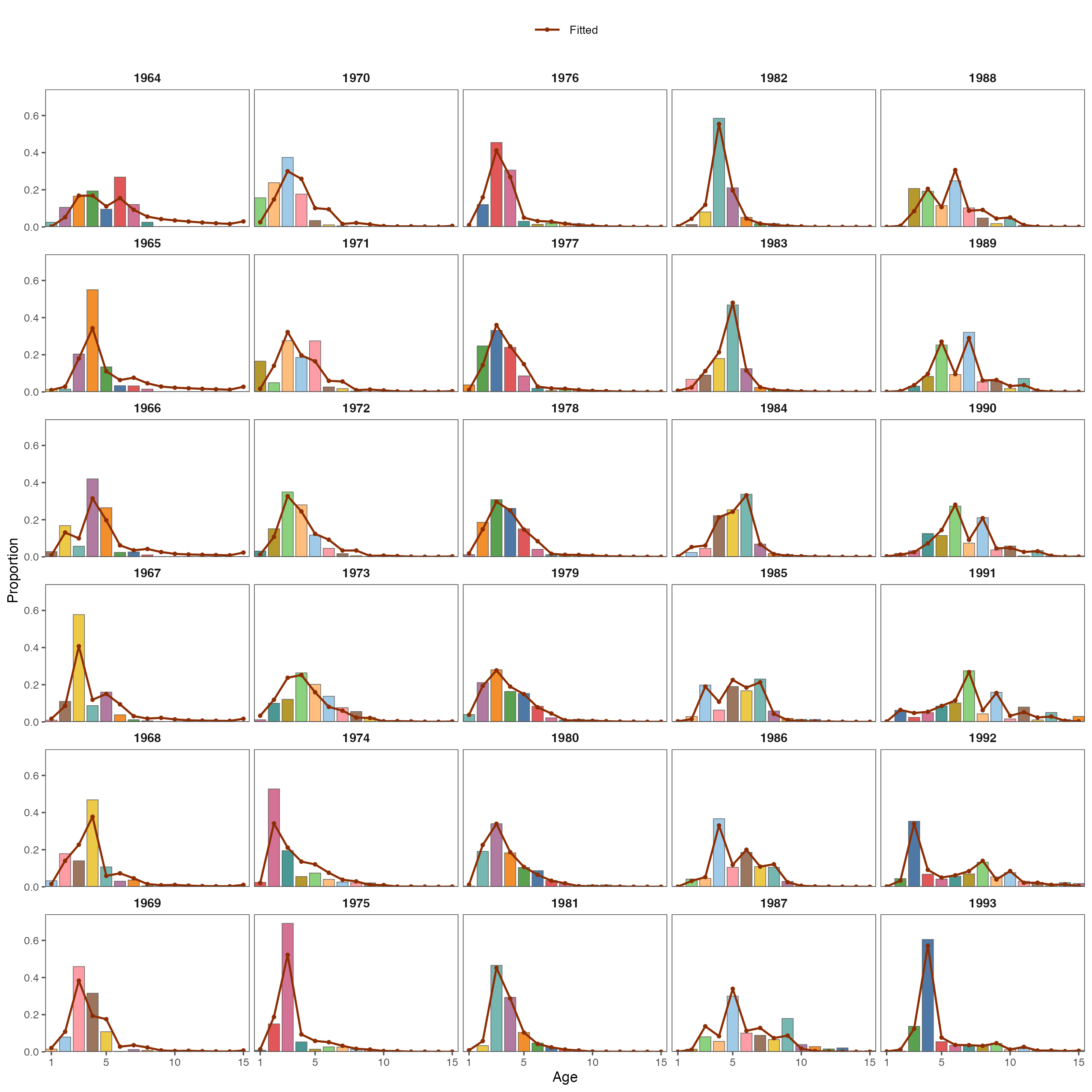
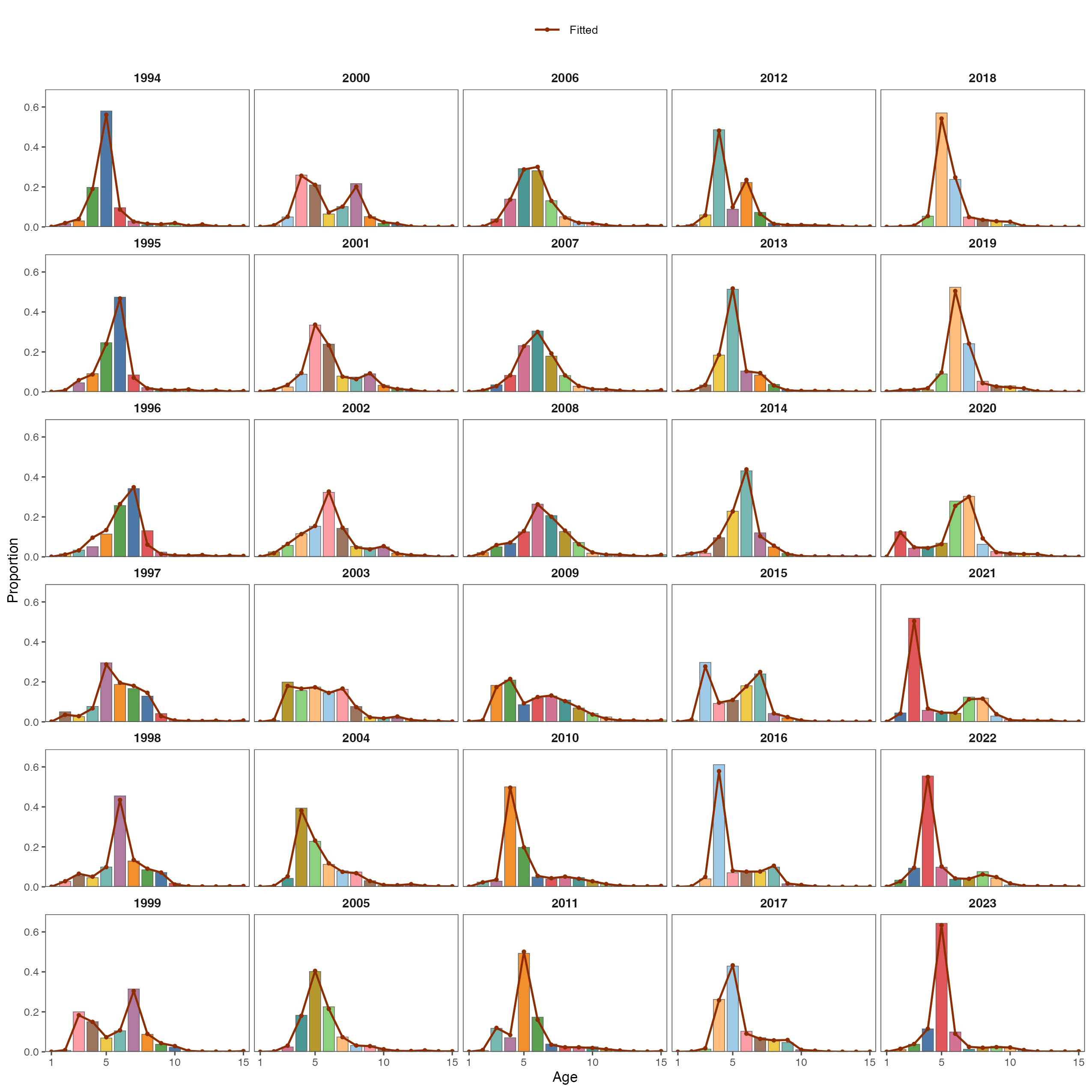
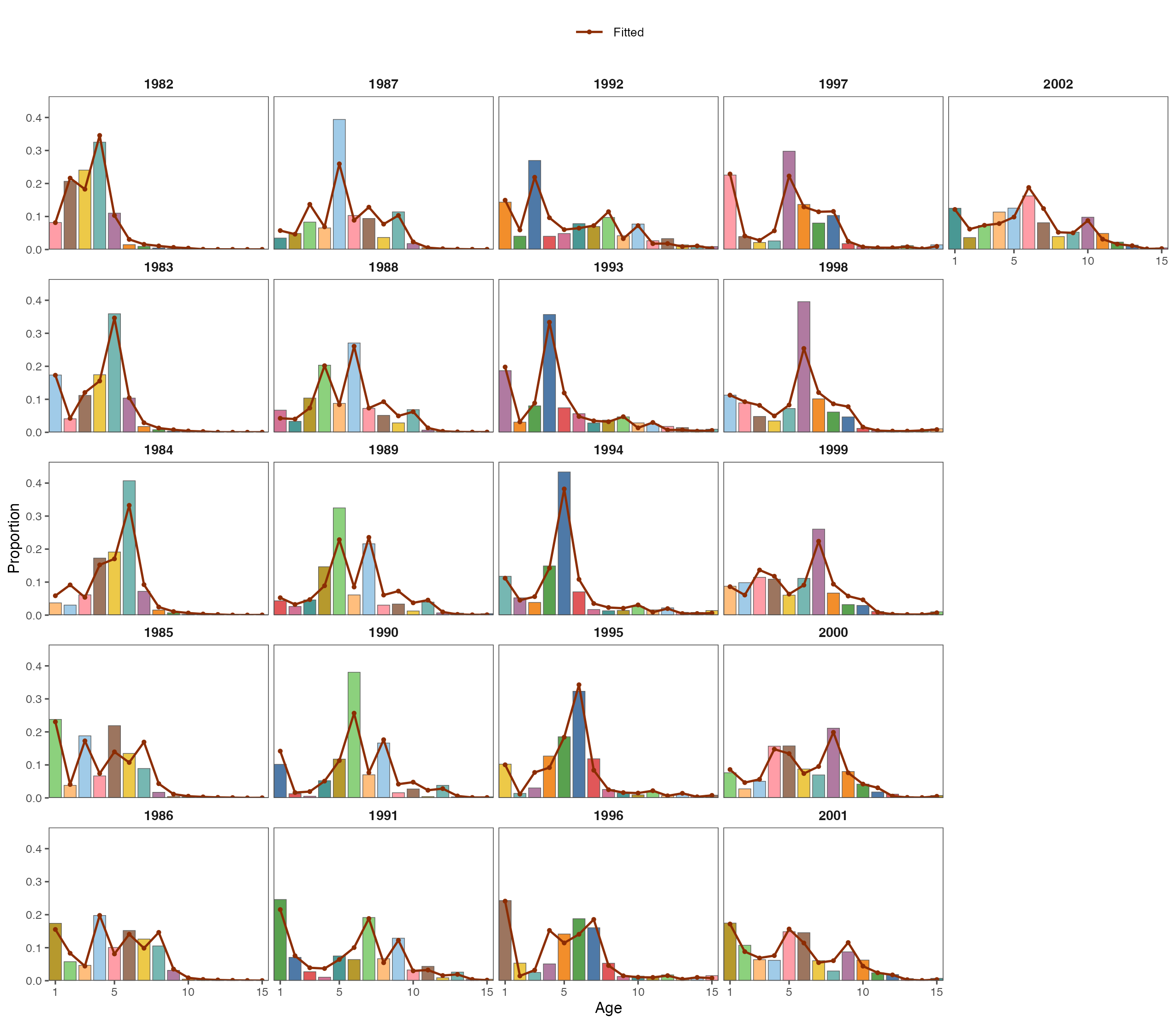
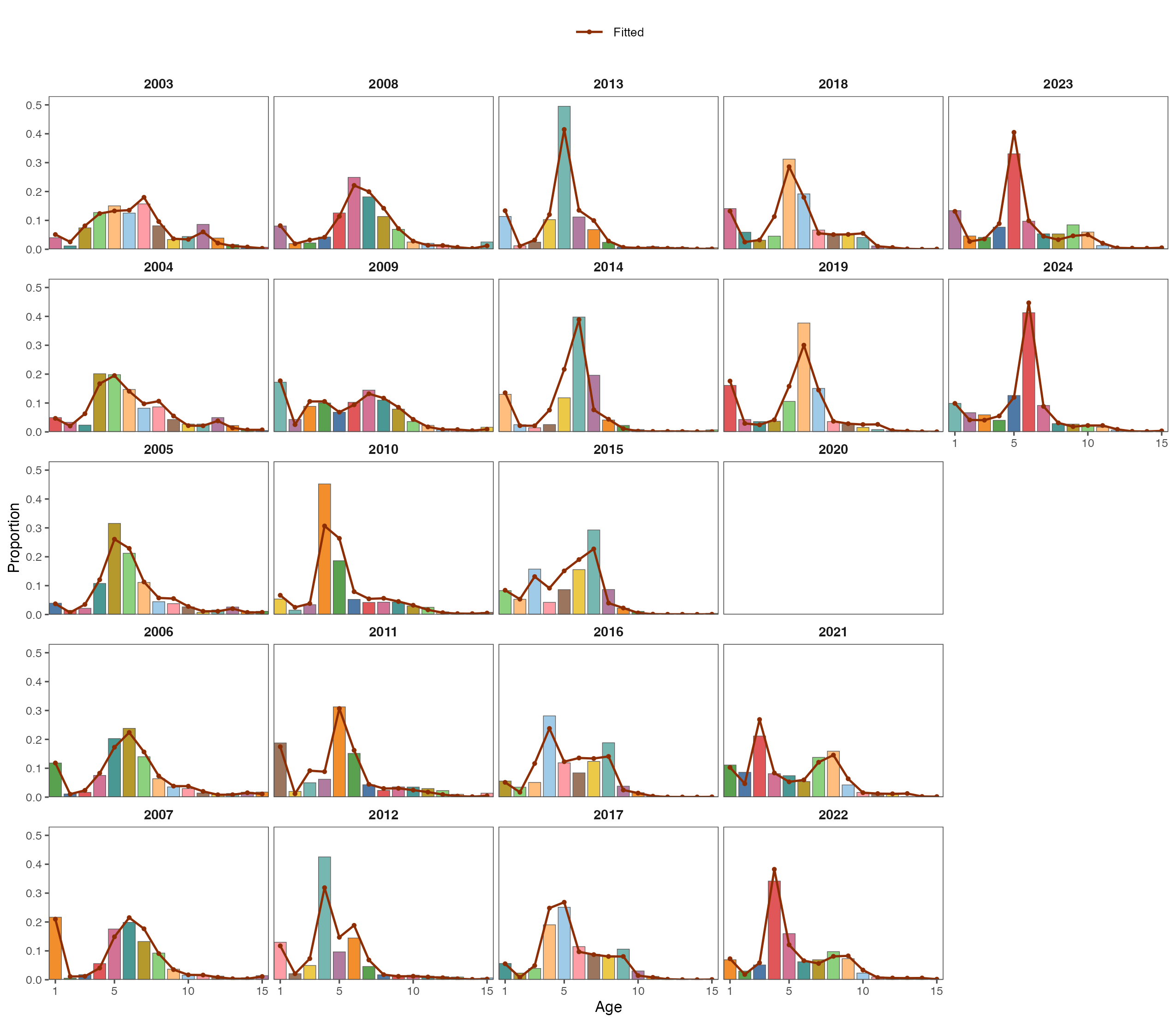
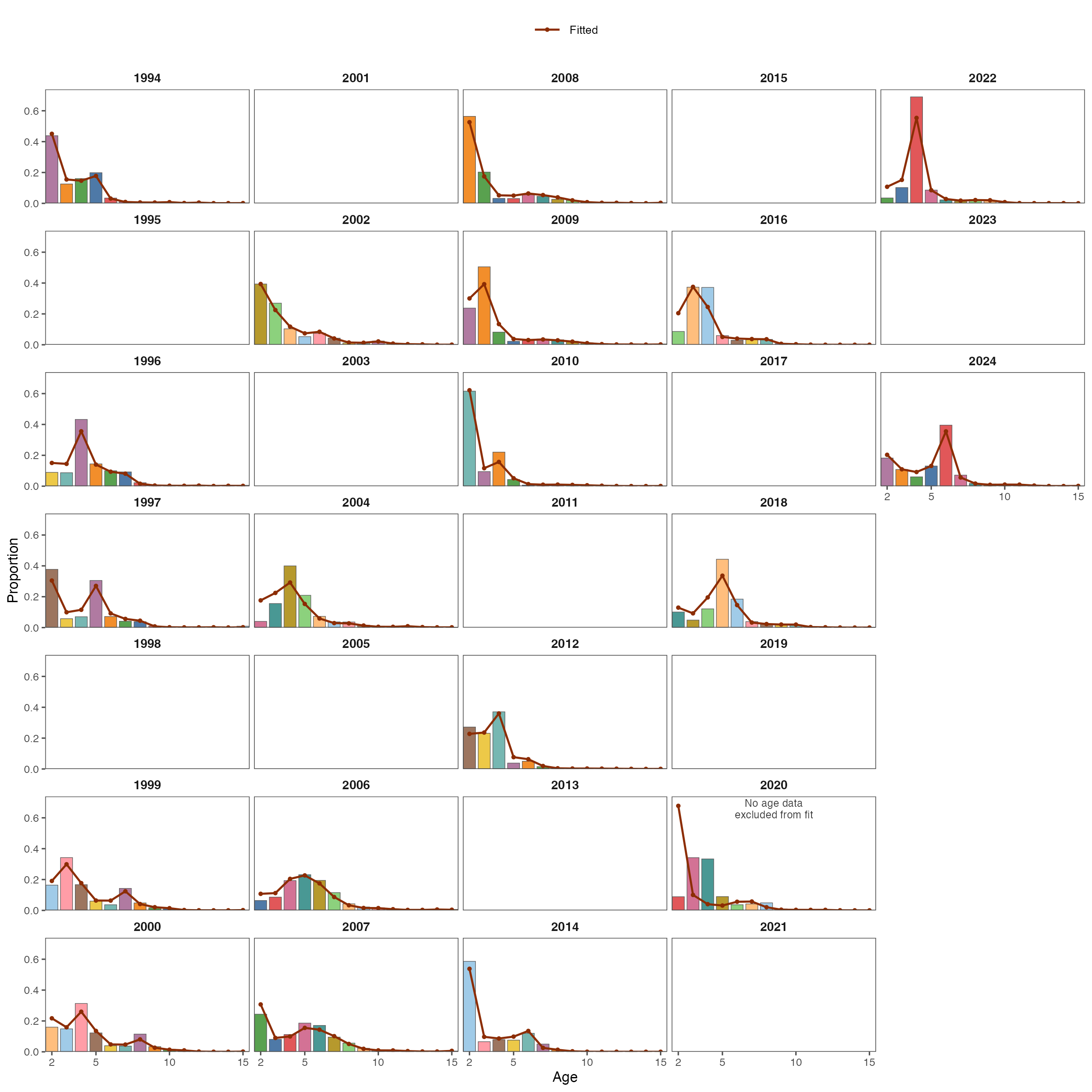
The annual age-composition panels compare observed proportions with fitted proportions for every sampling year available to Model 26.0. Panels proceed from the top to the bottom of each column and then continue at the top of the next column. A year without an age composition retains an empty panel. Fishery compositions span 1964–2023 (Figure 12 and Figure 13), BTS compositions span 1982–2024 (Figure 14 and Figure 15), and ATS compositions span 18 fitted survey years within the complete 1994–2024 panel sequence (Figure 16). The 2020 panel retains the workbook placeholder proportions for transparent review and labels them as excluded from fitting because no age-composition sample was collected.
Bar fill follows cohort, calculated as year minus age. The fixed 15-color cycle gives the 15 ages a distinct fill within a panel and retains the same color as a cohort ages across panels. For example, the 1988 cohort is red at age 2 in 1990, age 3 in 1991, and age 4 in 1992. The cycle repeats after 15 cohorts; the age position and year heading provide the primary identification, and color helps the reader follow diagonals through time.
The root-mean-squared difference between observed and fitted proportions is 0.024 for both the fishery and BTS. These direct fit plots show close agreement for many year-age combinations and identify local departures for the residual checks that follow. ATS compositions begin at age 2 because age 1 is represented by its separate abundance index. Across the 18 fitted ATS rows, the root-mean-squared difference is 0.029. The 2020 placeholder carries a likelihood sample size of zero and is omitted from this fit summary. The OSA section evaluates the same active ATS ages and fitted sampling events.
5.3.4 Diagnostics
The diagnostic sequence begins with one-step-ahead residuals for composition data, followed by dispersed starting values, simulated-data recovery, whole-index-fleet deletion, and retrospective peels. These tests address complementary questions: observation fit, sensitivity to starting values, recovery under known simulated data, influence of major survey streams, and stability as recent years are removed.
5.3.4.1 One-step-ahead residuals
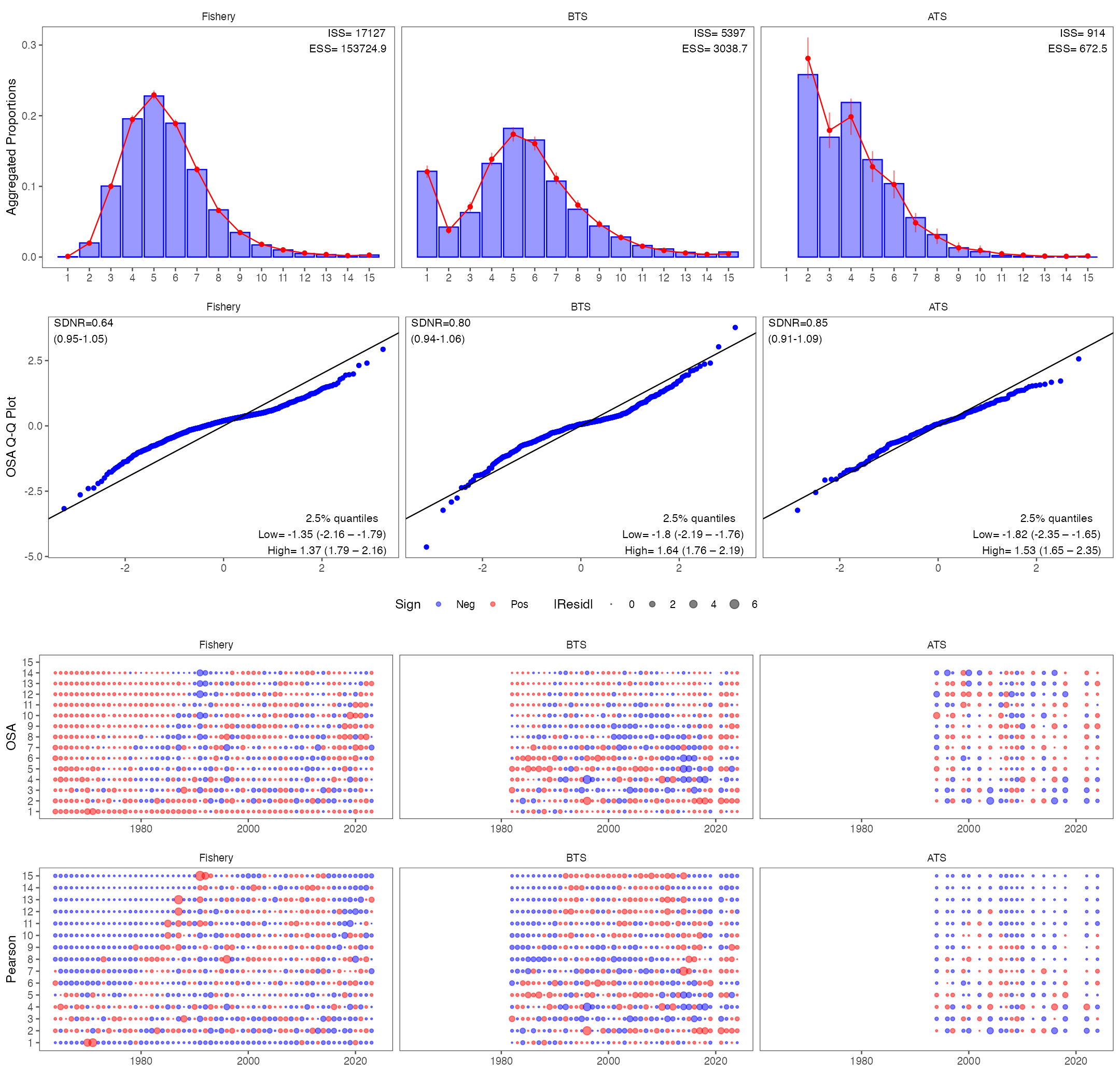
One-step-ahead (OSA) residuals compare each observed age proportion with its conditional prediction after the preceding age bins have been accounted for. Rceattle calculated the internal fishery and BTS residuals, and afscOSA version 0.0.1 produced the common AFSC plots and summaries. For ATS, afscOSA calculated the OSA residuals directly from ages 2–15, the ages that contribute to its composition likelihood. The N input came from the Rceattle Sample_size field used in the multinomial likelihood. It represents the likelihood sample size. The table reports the effective sample size separately.
The table and figure use the same composition rows retained by the afscOSA count conversion. The fishery and BTS retain every input year. ATS age 1 is zero in both the observed and fitted compositions, so its composition likelihood and diagnostics begin at age 2. Including the structural-zero column in a generic 15-bin residual sequence creates an artificial first residual and shifts the remaining ATS sequence. The corrected conversion uses the 14 contributing ages. ATS 2020 has no age-composition sample, carries a likelihood sample size of zero, and is excluded from both the Rceattle composition likelihood and the afscOSA conversion. The common display therefore uses the 18 fitted ATS years.
Each SDNR is below its expected interval: 0.638 for the fishery, 0.802 for BTS, and 0.849 for ATS (Table 7). The aggregate fits and residual bubbles show the age, year, and cohort locations of the remaining patterns (Figure 17). Interpretation emphasizes the aggregate fits and cells supported by appreciable predicted counts.
| Composition source | Years displayed | Residuals | SDNR | Expected interval | Likelihood sample-size total | Rounded count total | Effective sample size |
|---|---|---|---|---|---|---|---|
| Fishery | 60 | 840 | 0.638 | 0.952–1.048 | 17,147 | 17,127 | 153,725 |
| BTS | 42 | 588 | 0.802 | 0.943–1.057 | 5,403 | 5,397 | 3,039 |
| ATS | 18 | 234 | 0.849 | 0.909–1.091 | 929 | 914 | 673 |
afscOSA conversion.
5.3.4.2 Jitter test
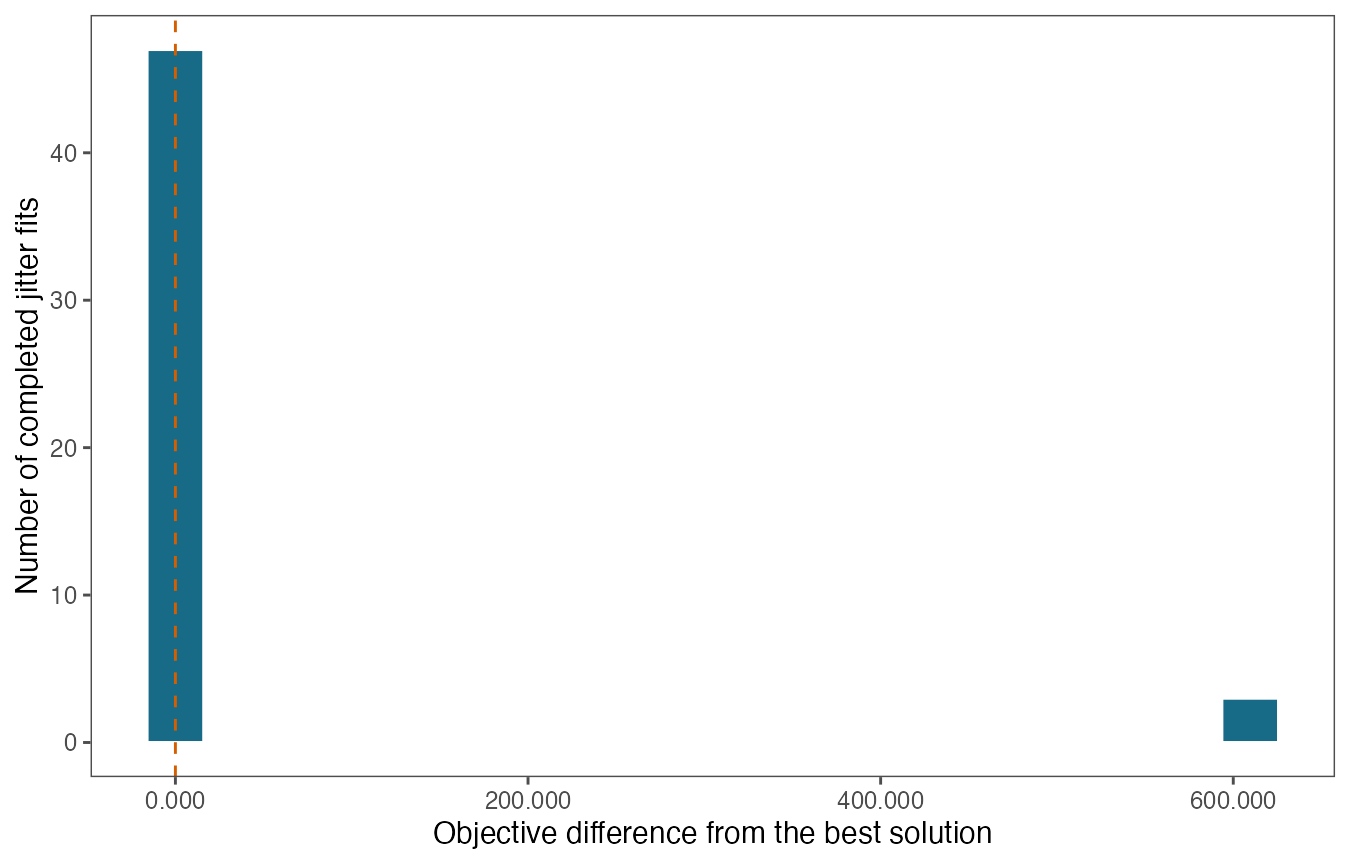
Fifty phased refits began from parameter values perturbed with standard deviation 0.2 and seed 20260831. All 50 completed with convergence status OK. Forty-seven returned to the best objective within 0.001. Three reached the same higher objective, approximately 609.6 units above the best value. The objective distribution and summary count show the 47 returns to the best solution and the three higher-mode fits (Figure 18; Table 8). This repeated higher solution identifies a second mode and supports retaining the two-stage fitting sequence and dispersed-start checks in routine work.
| Requested fits | Converged fits | Returned to best | Higher-mode fits | Largest objective difference |
|---|---|---|---|---|
| 50 | 50 | 47 | 3 | 609.6 |
5.3.4.3 Self-test
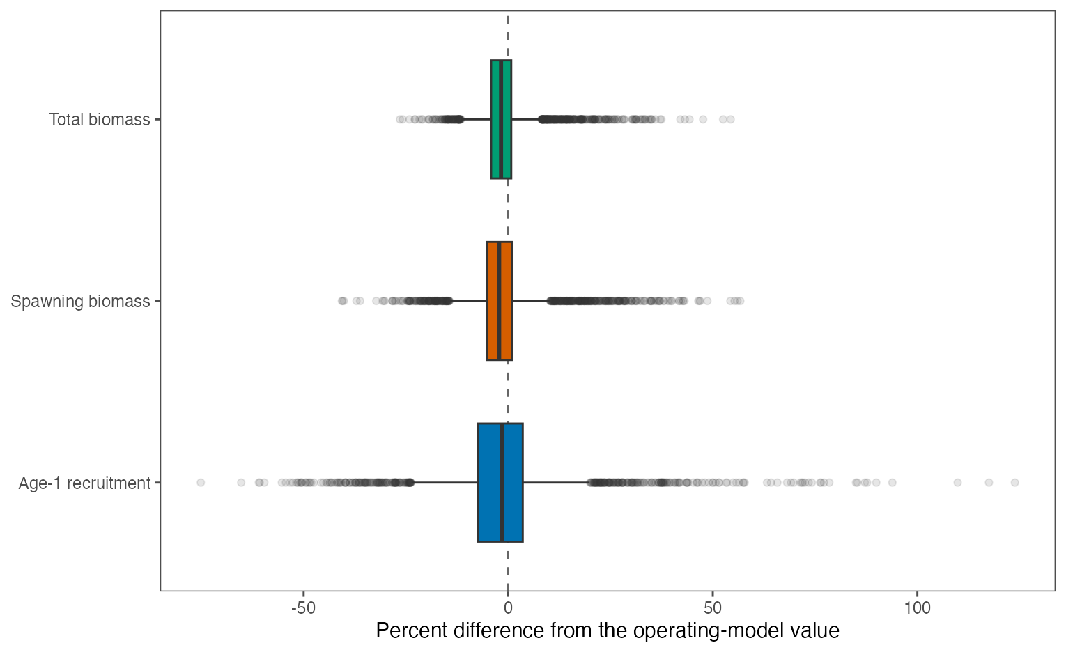
The self-test simulated 50 new observation sets from Model 26.0 and refitted each from the original pre-fit starting values. Recruitment deviations were held at their fitted realization, so this test measures recovery under new observation error. All 50 refits completed with convergence status OK; the largest maximum gradient was \(3.81\times10^{-4}\). Recruitment had the widest central 90% range and the largest mean absolute difference, while total biomass had the narrowest range and smallest mean absolute difference (Table 9; Figure 19).
The current simulator redrew some AVO and BTS index observations to retain positive values. Those simulated observations follow a positive-truncated distribution while the fitted bridge likelihood uses the corresponding normal form. The recovery summary therefore serves primarily as a fitting and coding check. A future observation-model sensitivity can align the fitted and simulated distributions directly.
| Quantity | Median difference | Mean absolute difference | Central 90% range |
|---|---|---|---|
| Age-1 recruitment | -1.49% | 9.76% | -23.31% to +23.31% |
| Spawning biomass | -2.21% | 6.27% | -13.49% to +17.85% |
| Total biomass | -1.75% | 4.81% | -9.58% to +13.29% |
5.3.4.4 Whole index-series sensitivity
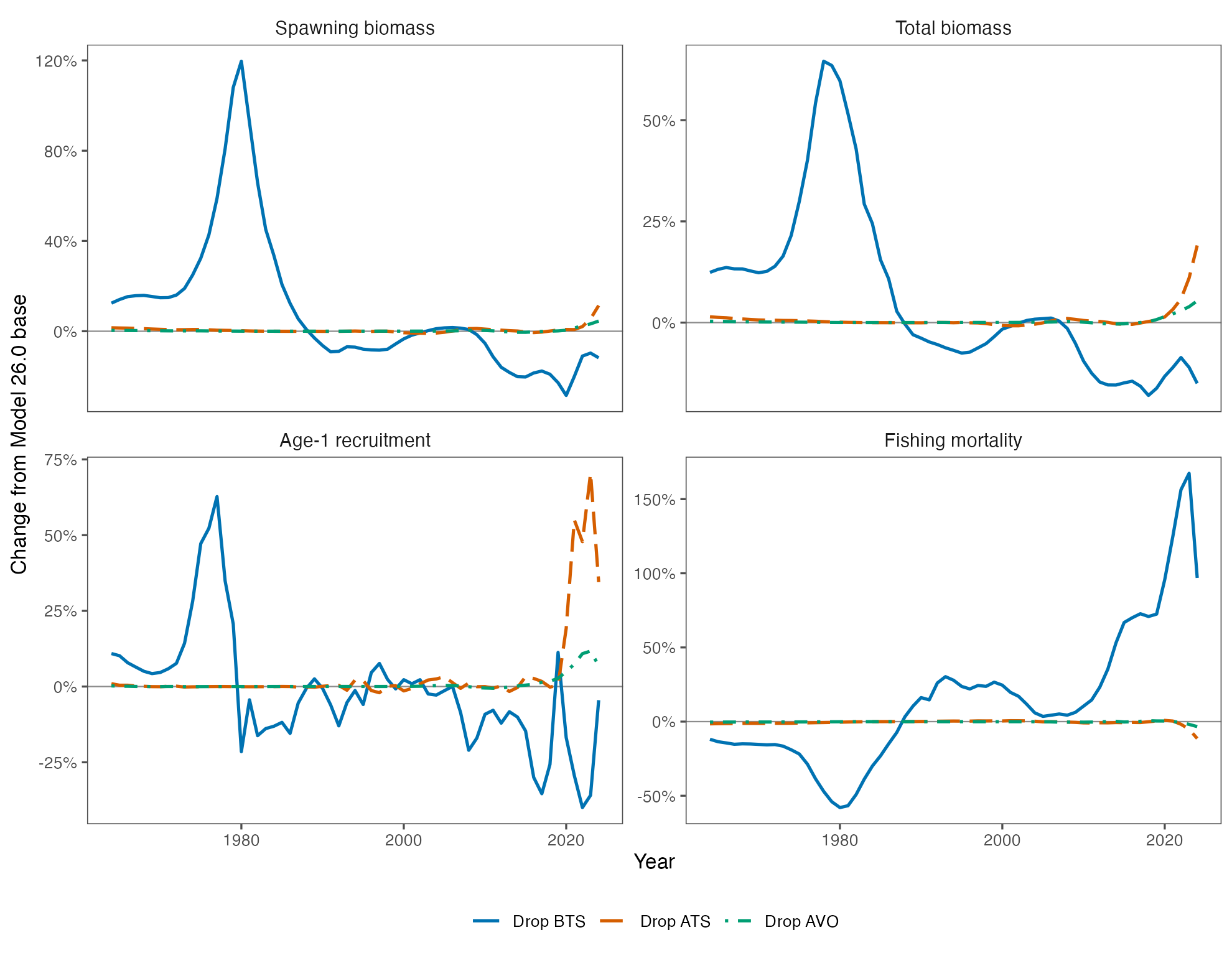
Three refits tested the influence of the complete BTS, ATS, and AVO fleets. Each fit started from the converged Model 26.0 estimates and retained the base configuration, including the non-parametric selectivity settings, fixed effects for recruitment deviations, and CPUE. Setting a fleet’s Fleet_type to Off removes its index and composition contributions from the likelihood. The ATS sensitivity also removed the separate ATS age-1 index fleet; the BTS age-1 fleet was already off in the base model. The objective values have different data contributions, so interpretation uses the trajectory changes rather than an objective or AIC comparison. The reproducible sensitivity script records this configuration.
All three refits completed with convergence status OK and positive-definite Hessians. Their maximum gradients ranged from \(2.09\times10^{-5}\) to \(3.89\times10^{-5}\). Dropping BTS had the greatest effect on population scale and fishing mortality: 2024 spawning biomass decreased 11.8%, total biomass decreased 15.0%, and fishing mortality increased 96.9%. Dropping ATS increased 2024 spawning biomass 11.4%, total biomass 19.1%, and recruitment 34.5%. Dropping AVO changed each 2024 quantity by less than 7% (Table 10).
The trajectories show the strong historical role of BTS and the increasing recent contribution of ATS, while AVO provides a smaller complementary signal (Figure 20). Whole-series deletion is an intentionally severe influence test. The result supports retaining all three survey streams and giving particular attention to BTS data preparation and availability in the operational update. The summary data and annual trajectories provide the reported values.
| Sensitivity | Index observations excluded | Composition years excluded | 2024 SSB change | 2024 total biomass change | 2024 recruitment change | 2024 fishing mortality change |
|---|---|---|---|---|---|---|
| Drop BTS | 42 | 42 | -11.8% | -15.0% | -4.5% | +96.9% |
| Drop ATS and ATS age-1 | 37 | 18 | +11.4% | +19.1% | +34.5% | -11.4% |
| Drop AVO | 18 | 0 | +4.5% | +5.4% | +6.9% | -3.4% |
5.3.4.5 Retrospective analysis
5.3.4.5.1 Configuration and primary results
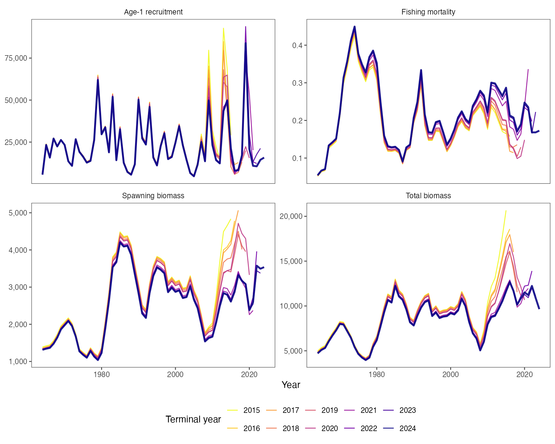
Nine peels ended in 2023 through 2015. The primary analysis follows the stream-specific lag rules used in the earlier retrospective analysis. Fishery age compositions retain their one-year lag, the ATS age-1 index retains its two-year lag, and the discontinued CPUE series continues to end in 1976. The remaining active index and composition series extend through the peel year when an observation exists. All 81 stream-by-peel checks reproduced these rules.
Each peel recalculates its data-based fishery-selectivity starting values and uses the same two-stage fitting sequence as the full Model 26.0 fit. The first stage establishes population and selectivity scale with annual selectivity changes held constant. The second stage estimates those annual changes. The terminal fishery and CPUE selectivity increment is fixed at zero, which carries the preceding-year selectivity-at-age curve into the terminal year. The largest terminal-to-preceding-year selectivity difference was \(6.7\times10^{-16}\). The retrospective script records the lag, convergence, and selectivity checks.
All nine peels completed with convergence status OK and positive-definite Hessians. The largest maximum gradient was \(2.01\times10^{-4}\).
The peels generally estimate greater spawning biomass, total biomass, and recruitment, together with lower fishing mortality, than the full model over the corresponding terminal years. Spawning biomass has the largest Mohn’s rho and the largest average relative revision, making it a central Model 26.0 evaluation priority (Table 11; Figure 21).
| Quantity | Mohn’s rho |
|---|---|
| Total biomass | 0.214 |
| Spawning biomass | 0.331 |
| Age-1 recruitment | 0.188 |
| Fishing mortality | -0.127 |
5.3.4.5.2 Sensitivity and evaluation
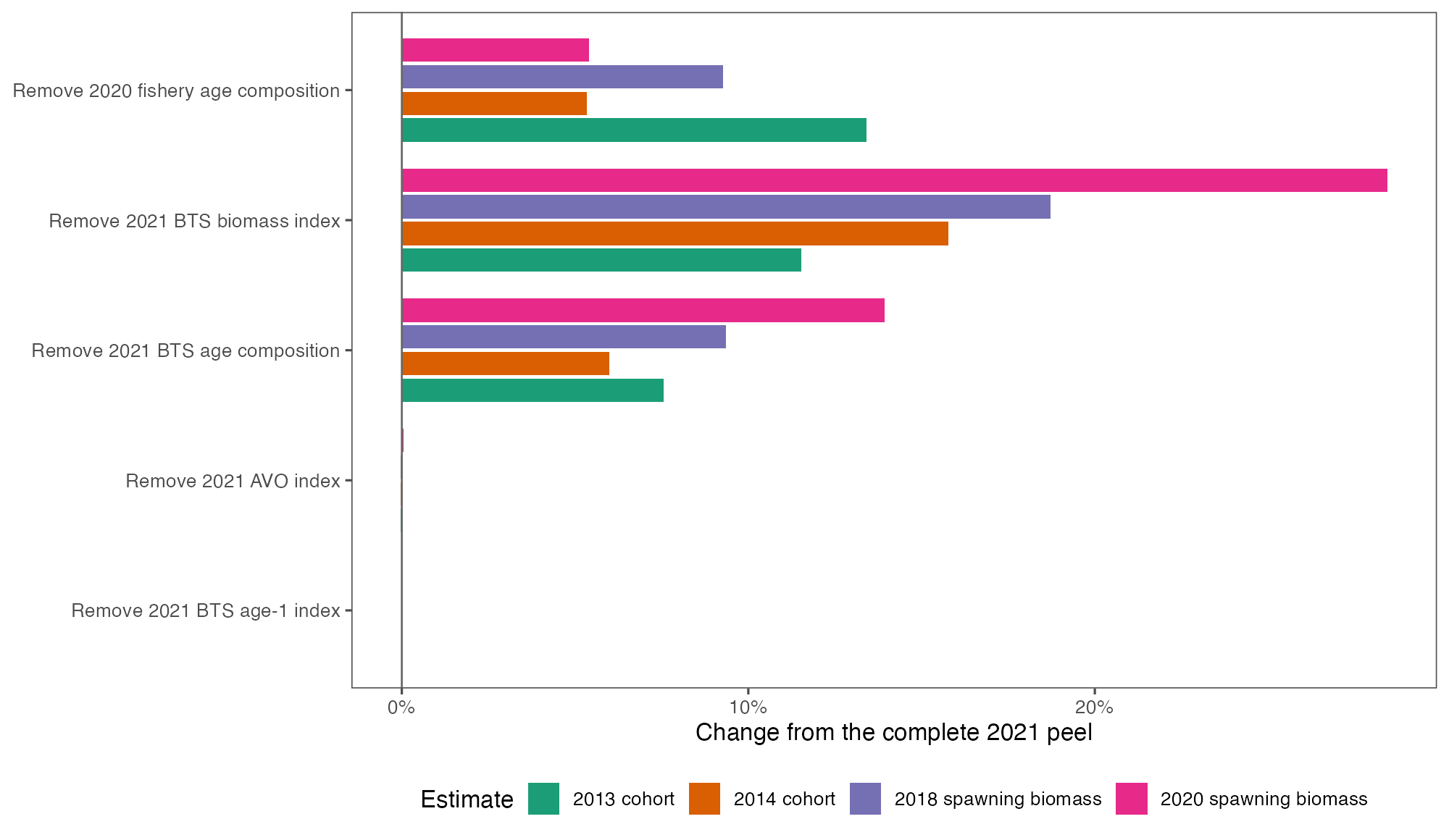
The data-sensitivity evaluation focuses on the main downward revision between the peels ending in 2020 and 2021. The same stream-specific lag rules identify five newly available observations: the 2020 fishery age composition and the 2021 BTS biomass index, BTS age composition, AVO index, and BTS age-1 index. Each controlled refit starts from the converged 2021-peel estimates, retains the 2021 parameter map, keeps DSEM disabled, and removes one observation block. This design measures the conditional influence of each new data block while holding the Model 26.0 structure constant. The data-sensitivity script records the observation inventory, block-deletion results, cumulative-addition results, and reproduction check.
All five block-deletion fits and six cumulative-addition fits completed with convergence status OK and positive-definite Hessians; the largest maximum gradient was \(1.34\times10^{-4}\). Removing the 2021 BTS biomass index had the largest effect on 2020 spawning biomass, increasing it by 28.4%, and increased the 2013 and 2014 cohort estimates by 11.5% and 15.8%. Removing the 2021 BTS age composition increased 2020 spawning biomass by 13.9%, while removing the 2020 fishery age composition increased the 2013 cohort by 13.4% and 2020 spawning biomass by 5.4%. The AVO and BTS age-1 index effects on these older cohorts and spawning biomass were negligible (Table 12; Figure 22).
The cumulative evaluation begins with the 2021 state and process dimensions and the observation availability of the 2020 peel. Adding the 2020 fishery age composition reduced the 2020 spawning-biomass difference from 47.5% to 29.1%, adding the 2021 BTS biomass index reduced it to 13.9%, and adding the 2021 BTS age composition brought it to within 0.05% of the complete 2021 peel. The AVO and BTS age-1 indices completed the sequence. The final step reproduced the complete 2021 objective and selected estimates exactly. Together, the removal and addition tests identify the fishery age composition and BTS data as the principal signals associated with this retrospective revision, with the BTS biomass index providing the largest single influence on spawning biomass.
| Data block removed | 2013 cohort change | 2014 cohort change | 2020 SSB change | Maximum gradient |
|---|---|---|---|---|
| 2020 fishery age composition | +13.4% | +5.3% | +5.4% | \(4.25\times10^{-5}\) |
| 2021 BTS biomass index | +11.5% | +15.8% | +28.4% | \(4.90\times10^{-5}\) |
| 2021 BTS age composition | +7.5% | +6.0% | +13.9% | \(6.24\times10^{-5}\) |
| 2021 AVO index | -0.02% | -0.03% | +0.05% | \(4.31\times10^{-5}\) |
| 2021 BTS age-1 index | 0.0% | 0.0% | 0.0% | \(4.12\times10^{-5}\) |
5.3.5 Projections
The projection uses spmR version 0.3.0 and the validated Standard Projection Model workflow. The projection runner and input writer transfer the current Model 26.0 population state, annual recruitment, biological schedules, and recent fishing pattern into the pm.prj format. The projection uses the arithmetic mean fishery selectivity-at-age and fishing mortality from 2020–2024; mean fishing mortality over those years is 0.1984.
5.3.5.1 Standard alternatives
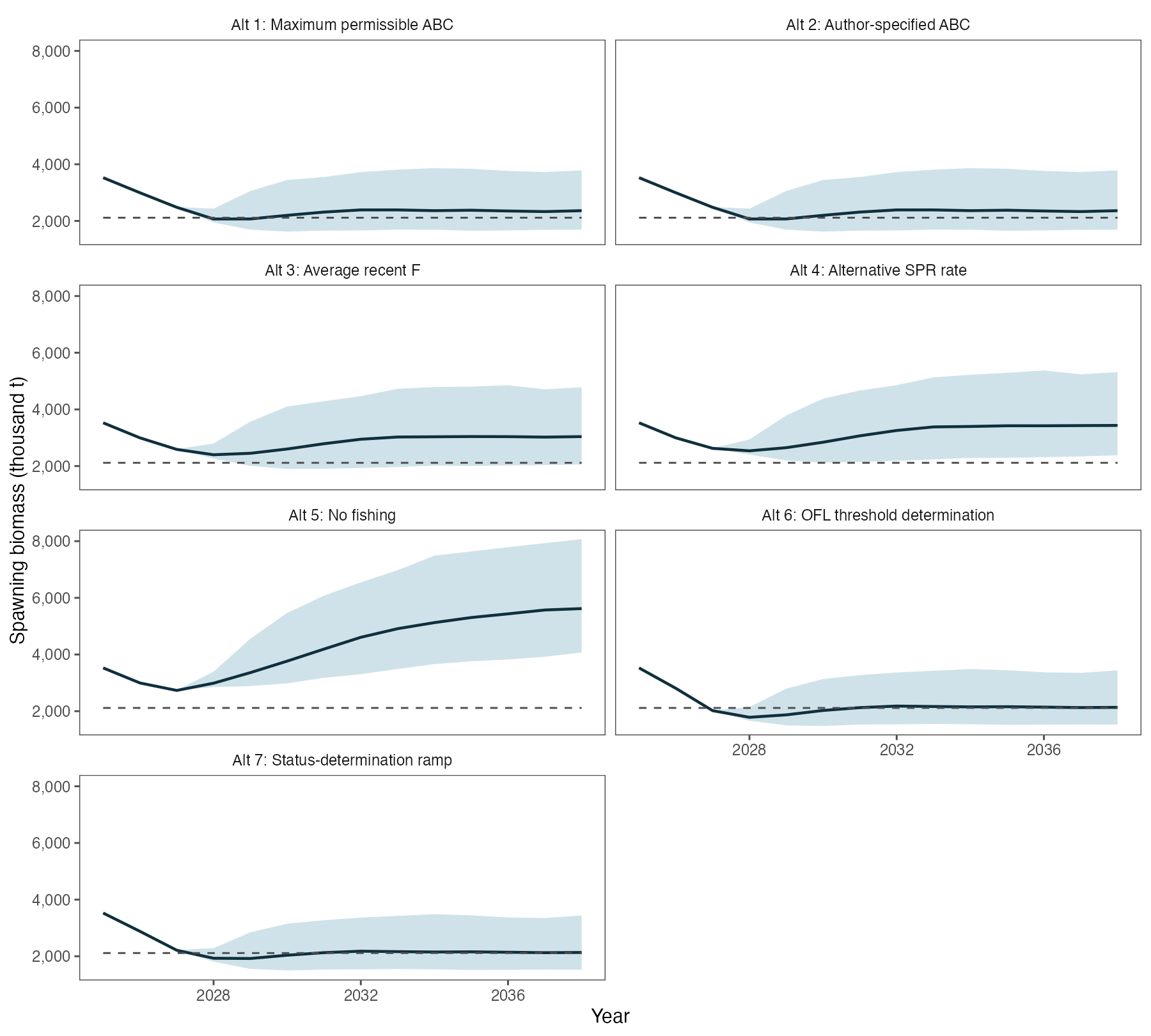
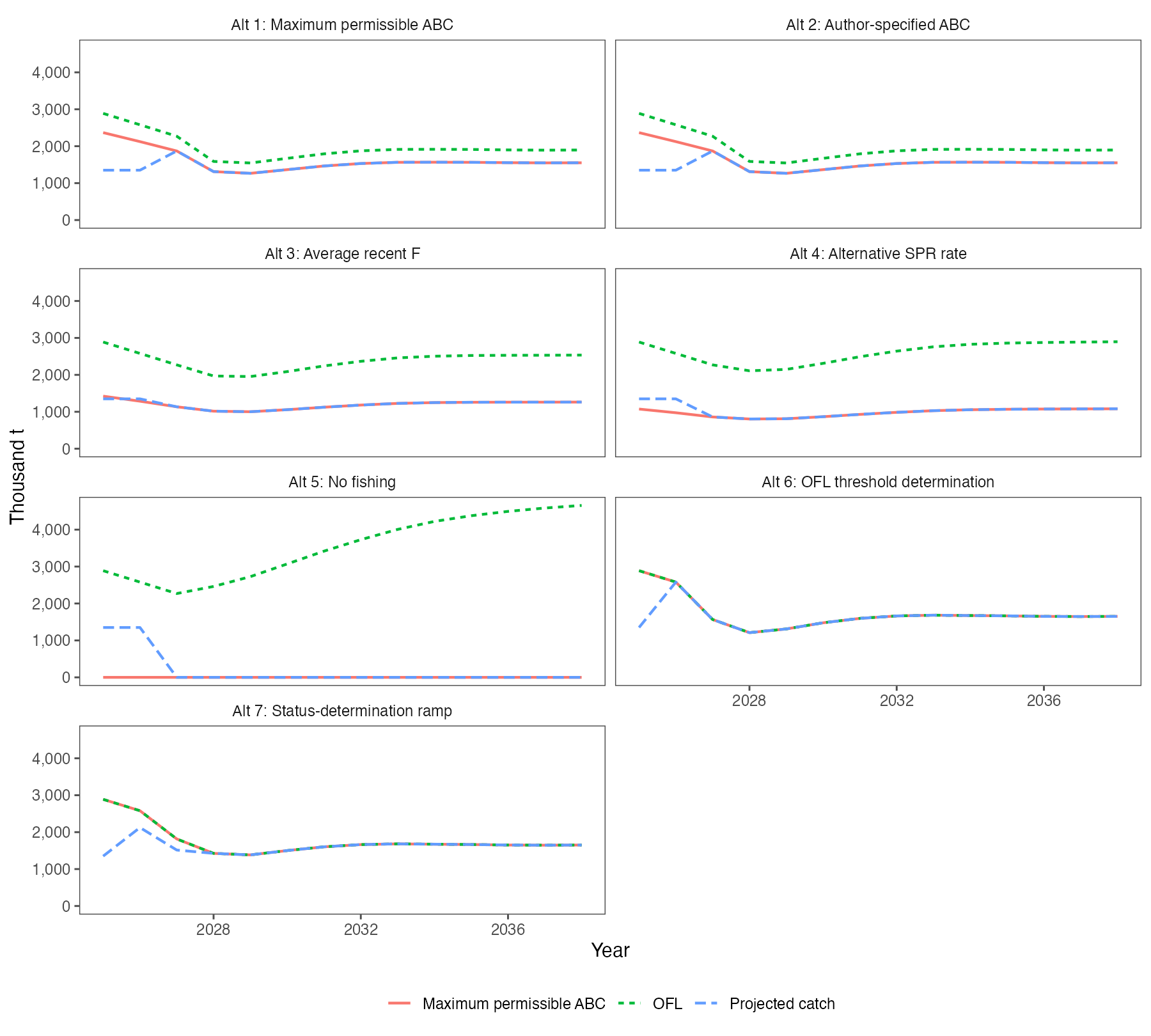
The seven alternatives use 1,000 simulations over 14 projection years beginning in 2025. Catch is fixed at 1,350 thousand t in 2025 and 2026, so the alternatives first separate in 2027. These Model 26.0 results are intended to just demonstrate the linkage with the standard Tier 3 projection model. ABC and OFL recommendations and status determinations will be available when the new data are updated for the SSC’s December 2026 consideration.
The 2027–2028 comparison keeps spawning biomass at or above the \(B_{35\%}\) proxy under Alternatives 1–5. Alternative 6 is below the proxy in both years, and Alternative 7 moves below it in 2028. Projected catch, ABC, and OFL share the fixed-catch assumptions in 2025 and 2026 and then follow the rules for each alternative (Table 13; Figure 23; Figure 24).
| Alternative | Year | Catch | ABC | OFL | SSB | F | B/B35% |
|---|---|---|---|---|---|---|---|
| 1 | 2027 | 1,870 | 1,870 | 2,270 | 2,483 | 0.35 | 1.17 |
| 1 | 2028 | 1,312 | 1,312 | 1,587 | 2,118 | 0.31 | 1.00 |
| 2 | 2027 | 1,870 | 1,870 | 2,270 | 2,483 | 0.35 | 1.17 |
| 2 | 2028 | 1,312 | 1,312 | 1,587 | 2,118 | 0.31 | 1.00 |
| 3 | 2027 | 1,135 | 1,135 | 2,270 | 2,589 | 0.20 | 1.22 |
| 3 | 2028 | 1,016 | 1,016 | 1,969 | 2,451 | 0.20 | 1.16 |
| 4 | 2027 | 859 | 859 | 2,270 | 2,626 | 0.15 | 1.24 |
| 4 | 2028 | 805 | 805 | 2,110 | 2,589 | 0.15 | 1.22 |
| 5 | 2027 | 0 | 0 | 2,270 | 2,733 | 0.00 | 1.29 |
| 5 | 2028 | 0 | 0 | 2,462 | 3,041 | 0.00 | 1.44 |
| 6 | 2027 | 1,566 | 1,566 | 1,566 | 2,019 | 0.37 | 0.96 |
| 6 | 2028 | 1,211 | 1,211 | 1,211 | 1,831 | 0.34 | 0.87 |
| 7 | 2027 | 1,515 | 1,815 | 1,815 | 2,214 | 0.32 | 1.05 |
| 7 | 2028 | 1,425 | 1,425 | 1,425 | 1,978 | 0.36 | 0.94 |
spmR results for 2027 and 2028. Catch, ABC, OFL, and SSB are rounded simulation means in thousand t.
5.3.5.2 Fixed-catch sensitivity
An additional Alternative 2 run fixes catch at 1,300 thousand t from 2025 through 2032. Mean spawning biomass remains above the \(B_{35\%}\) proxy through the displayed fixed-catch period. The displayed \(B/B_{35\%}\) values remain above one, reaching 1.12 in 2028 and 1.25 in 2032 (Table 14).
| Year | Catch | ABC | OFL | SSB | F | B/B35% |
|---|---|---|---|---|---|---|
| 2025 | 1,300 | 2,368 | 2,888 | 3,533 | 0.180 | 1.67 |
| 2026 | 1,300 | 2,138 | 2,597 | 3,023 | 0.199 | 1.43 |
| 2028 | 1,300 | 1,590 | 1,917 | 2,372 | 0.268 | 1.12 |
| 2030 | 1,300 | 1,463 | 1,790 | 2,450 | 0.308 | 1.16 |
| 2032 | 1,300 | 1,597 | 1,970 | 2,648 | 0.313 | 1.25 |
5.3.6 Exploratory DSEM recruitment pathways
The Dynamic Structural Equation Model (DSEM) analysis links recruitment to a small set of prespecified environmental pathways while retaining the Model 26.0 assessment structure. It uses the same Rceattle 5.23.0 branch snapshot. The four models share the same observation years, missing-value pattern, standardization, and time-series treatment of the two environmental indices.
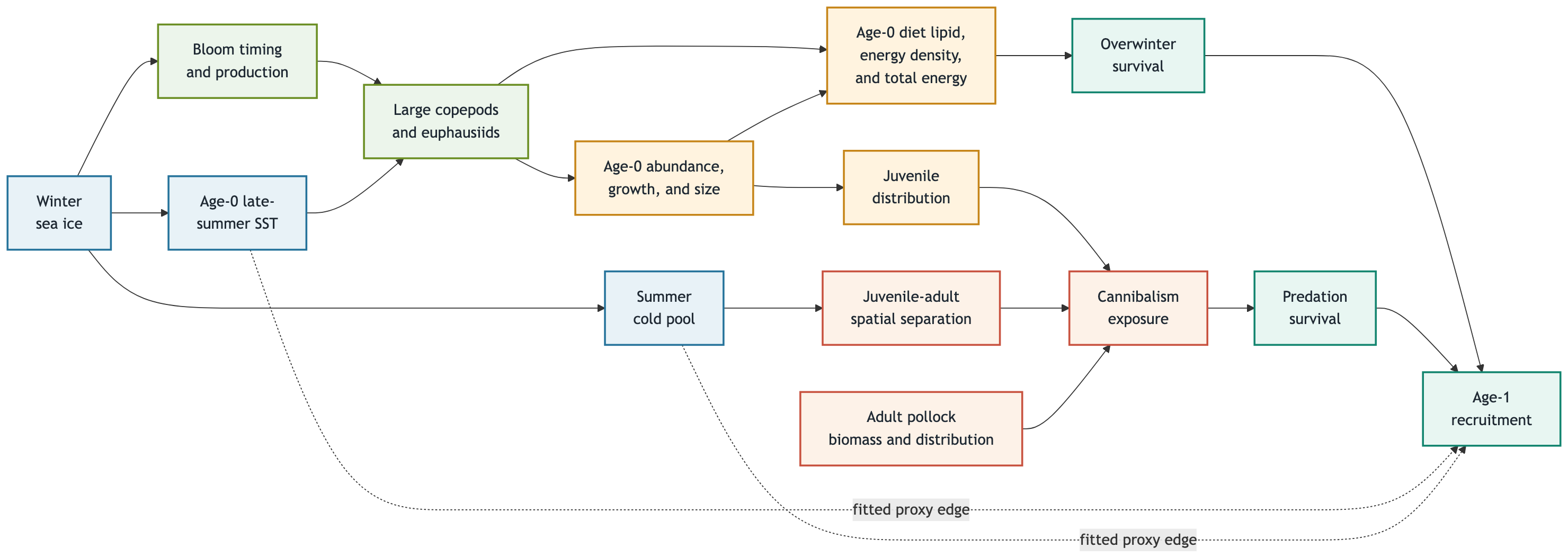
The response is age-1 recruitment. Late-summer sea-surface temperature (SST) is aligned with the cohort’s age-0 year. Cold-pool extent is aligned with the following age-1 calendar year. SST represents a broad energetic-condition pathway, while cold-pool extent represents a possible spatial-separation and cannibalism pathway. The conceptual graph keeps the biological steps visible even though the fitted examples use direct proxy paths (Figure 25).
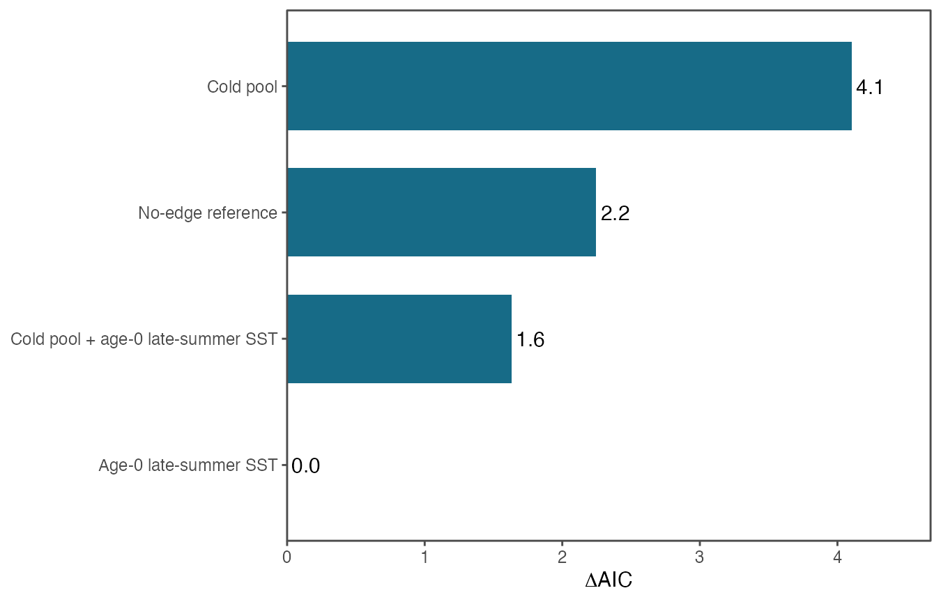
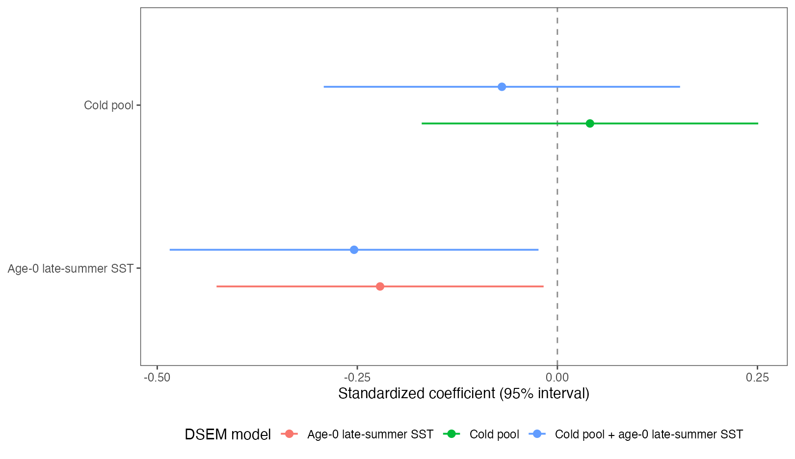
All four DSEM fits completed with positive-definite Hessians and convergence status OK. Fit AIC favored the DSEM model with age-0 late-summer SST. The combined model was 1.63 AIC units higher, the no-edge reference was 2.25 units higher, and the cold-pool model was 4.10 units higher (Figure 26; Table 15).
The SST pathway is negative in both models that include it, with intervals below zero. The cold-pool pathway is smaller and its interval spans zero in both models (Figure 27; Table 16). These results describe an in-sample association that is consistent with the proposed energetic pathway. Direct measurements of fall age-0 energy, prey quality, overwinter survival, and juvenile-adult overlap will provide the stronger next tests of the biological mechanism.
The diagnostics and DSEM results support continued Model 26.0 development. The close bridge trajectories and complete convergence provide a strong implementation basis. The OSA dispersion, repeated higher jitter mode, and positive spawning-biomass retrospective pattern define the next evaluation priorities. The ESP framework in Appendix 2 organizes the additional indicator and mechanism work.
| DSEM specification | Delta AIC | Reduction in unexplained recruitment variation |
|---|---|---|
| Age-0 late-summer SST | 0.00 | 10.5% |
| Cold pool + age-0 late-summer SST | 1.63 | 12.0% |
| No-edge reference | 2.25 | 0.0% |
| Cold pool | 4.10 | 0.3% |
| Model | Recruitment pathway | Estimate | 95% interval |
|---|---|---|---|
| Cold pool | Cold pool | 0.041 | -0.169 to 0.251 |
| Age-0 late-summer SST | SST | -0.222 | -0.426 to -0.017 |
| Combined | Cold pool | -0.069 | -0.292 to 0.153 |
| Combined | SST | -0.254 | -0.484 to -0.024 |
6 Conclusion
Model 26.0 provides a reproducible Rceattle implementation of the EBS pollock assessment. It closely follows the Model 23.2 bridge, passes the stated convergence and simulated-data recovery checks, carries the assessment state into the standard Tier 3 projection model, and makes the full analysis available through documented R workflows. The whole-index-fleet sensitivities show that BTS supplies the strongest information about population scale and fishing mortality, ATS contributes increasingly to recent biomass and recruitment, and AVO provides a smaller complementary signal. These patterns are consistent with the roles and lengths of the three survey series.
Rceattle is also being used to develop the Gulf of Alaska (GOA) pollock assessment, and the companion comparison successfully reran the GOA base model through its numerical fit checks. The GOA application estimates recruitment and changes in survey catchability within the fitted model, whereas the EBS application emphasizes translation of the established ADMB structure and a separate spmR projection handoff. Together, the applications show how Rceattle can support stocks with different survey histories and assessment structures. They also provide a shared basis for pinning software and input versions, recording which observations enter each fit, applying common fit and retrospective checks, and testing the projection handoff. Stock-specific surveys, age ranges, and selectivity choices remain central to each assessment while the shared Rceattle platform supports consistent and transparent evaluation across both regions.
The diagnostic results also define a practical operational checklist. The production run should retain the two-stage fitting sequence and multi-start evaluation, repeat the OSA and lag-preserving retrospective analyses, review BTS inputs closely, and carry the fitted state into the validated spmR projection workflow. The operational specification should keep DSEM disabled (DSEM = NULL); the environmental pathways and SparseNUTS work remain separate research evaluations.
The combined bridge, convergence, self-test, index-sensitivity, retrospective, and projection evidence supports a recommendation that the Plan Team and SSC adopt Model 26.0 for producing EBS pollock management advice in November and December 2026. The updated-data run will provide the ABC, OFL, and stock-status results for that review. Model 23.0 provides continuity until the review bodies complete this transition.
References
Appendices
Appendix 1: Main SSC comments and responses
A funding lapse ended preparation of the November and December 2025 EBS pollock SAFE package. The October 2025 SSC comments therefore carry forward to the 2026 assessment cycle for formal response. The responses below describe the planned work for 2026 and later years.
Current status
- The next assessment needs to trace the 2025 RTMB starting model back to the 2024 ADMB source, along with updated survey data, 2025 FT-NIRS ages, the comparison of traditional and FT-NIRS ages, model names, and the document archive.
- Work continues on Rceattle, SPoRC, natural mortality, selectivity, and age-composition weighting in response to the SSC comments.
- Current analyses address Russian catches and the recruitment penalty for the 2018 year class.
- Work on the revised AVO index depends on completion and review of the new uncertainty analysis.
Completion of an SSC response requires the analysis, results, and explanation for review. Current research contributes evidence toward that completion.
Earlier responses to 2024 SSC comments
The responses below were on the previous version of the SSC response page and retain their original scientific claims. Confirm these claims against the completed analyses and assessment record before citing them as final 2025 results.
Dynamic Species Environment Models (DSEM) and recruitment mechanisms
The SSC recommended further exploration of DSEM to reconcile contrasting signals such as record larval biomass in 2024, low age-0 abundance, chronically low condition, and increasing adult biomass.
In 2025, exploratory DSEM analyses continue under the ESR framework and remain outside the current assessment. The Recruitment section presents anomalous recruitment indicators for context.
2026 activity: The Rceattle application presents the DSEM analysis together with preliminary ESP work.
Pollock cannibalism index
The SSC requested extrapolation of the index to biomass consumed.
For 2025, the index is updated. Work continues toward final biomass-consumed estimates as a development priority.
Tier 1 vs. Tier 3 classification
The SSC supported Tier 3 classification given reliance on priors and limited data at low stock sizes.
The 2025 assessment maintains Tier 3a status and focuses its calculations on that tier, consistent with SSC guidance.
Multispecies model outputs
The SSC encouraged use of time-varying mortality or consumption estimates from the multispecies model, noting its strategic role in climate planning.
In 2025, multispecies outputs remain under review for potential use in ESP indicators and future assessment development.
Biological observations
The SSC noted low weight-at-age and condition in recent years and emphasized the importance of the 2018 year class.
The 2025 BTS confirms condition remains below average. The 2018 year class continues to dominate spawning biomass but shows expected decline as it ages out of the population.
Selectivity assumptions
The SSC supported the use of the five-year moving average selectivity for projections.
This method is retained in 2025, with updated retrospective diagnostics.
Model status and diagnostics
The SSC endorsed Model 23.0, Tier 3a classification, and ABC equal to the maximum permissible.
Model 23.0 is retained for 2025 with updated data inputs. Tier 3a status and ABC recommendations remain as supported by the SSC.
Additional recommendations
- State-space approach (TMB/RTMB): exploratory work is ongoing.
- Russian proportion/movement: work continues to develop updated estimates.
- FT-NIR age validation: further evaluation continues in preparation for integration.
- Recruitment penalty (2018 cohort): sensitivity analyses are included; discussion of penalty influence is provided.
Stock-Recruitment relationship
The SSC noted reduced influence under Tier 3, but stressed unbiased estimation of recruitment deviates and transparent use of steepness priors.
The recruitment bias correction is set to zero; steepness priors remain meta-analysis based. The 2025 assessment presents the Tier 3 analysis.
Documentation request
The SSC requested that the September 2024 SRR document be included as an appendix or linked.
The document has been added as Appendix X in this SAFE.
SSC 2024 comments and 2025 responses
The retained response matrix summarizes how the 2025 work addressed each 2024 SSC comment and identifies topics that continue into the current cycle.
| SSC comment | 2025 response |
|---|---|
| Explore use of DSEM for pollock recruitment anomalies | Recruitment section presents the anomalies; exploratory analyses continue toward future integration. |
| Extrapolate cannibalism index to biomass consumed | Index updated; extrapolated biomass estimates continue in development toward final review. |
| Tier 1 vs. Tier 3 classification | Maintained Tier 3a classification and focused calculations on that tier. |
| Use multispecies model outputs (time-varying M, consumption) | Multispecies outputs remain under review for ESP and future assessment use. |
| Biological observations (low condition, 2018 year class) | 2025 BTS confirms below-average condition; 2018 cohort still dominant but declining. |
| Use of five-year moving average selectivity | Retained for 2025 projections; retrospective diagnostics updated. |
| Endorse Model 23.0, Tier 3a, ABC=max permissible | Continued use of Model 23.0; Tier 3a classification; ABC set equal to maximum permissible. |
| Recommendations: state-space approach, Russian distribution, FT-NIR, recruitment penalty | State-space exploration and FT-NIR evaluation continue; work is developing updated Russian estimates; sensitivity runs describe the penalty influence. |
| Stock-recruitment relationship | The 2025 assessment focuses on recruitment deviations with zero bias correction; the steepness prior remains meta-analysis based. |
| Add Sept 2024 SRR document as appendix | Document included as Appendix X. |
Appendix 2: Draft EBS pollock ESP development framework
This appendix provides a working structure for an eastern Bering Sea pollock Ecosystem and Socioeconomic Profile (ESP). It separates the concise assessment development results in Section 5.3 from the broader indicator synthesis, evidence trail, and update cycle needed for a complete ESP. The headings below can be expanded as current-year ecosystem and socioeconomic products become available.
| ESP component | EBS pollock content | Current development status |
|---|---|---|
| Executive summary | Management relevance, principal ecosystem signals, socioeconomic conditions, and key data needs | Complete after the annual indicator assessment |
| Introduction and justification | Purpose, review history, focal population responses, and intended management use | Initial justification recorded; team review planned |
| Data | Assessment states, physical indices, plankton and prey indices, age-0 condition, predation and overlap products, and socioeconomic series | Core inventory assembled; biological mediators continue to expand |
| Indicator synthesis | Life-history table, conceptual pathways, and mechanism table | Draft structure and initial recruitment graph available |
| Proposed indicators | Small set selected by mechanism, timing, record length, uncertainty, and annual availability | SST and cold pool illustrate the workflow; age-0 energy and prey remain priorities |
| Indicator assessment | Current condition, trends, uncertainty, and plain-language interpretation | Update with current-year ESP and Ecosystem Status Report products |
| Indicator analysis | Common-data DSEM comparisons, pathway estimates, prediction checks, and scientific sign checks | Four current-branch DSEM fits presented in Section 5.3 |
| Data gaps and priorities | Age-0 energy, prey lipid and abundance, bloom-prey timing, overlap, and observation error | Priorities identified for team confirmation and annual production |
| Conclusion and management use | Role of each indicator in recruitment modeling, risk assessment, or monitoring | Complete after validation and review |
The framework assigns every ESP component a purpose and current development status, keeping the pending annual synthesis and review steps visible (Table 17).
Executive summary
Summarize the current ecosystem and socioeconomic conditions after the annual indicator assessment is complete. Distinguish indicators that improve prediction from those that provide management context.
Introduction and justification
The ESP will connect ecosystem and fishing-community conditions with the assessment quantities used to evaluate pollock status and risk. Age-1 recruitment is the initial focal population response because early survival links physical conditions, prey, age-0 condition, overwinter survival, and cannibalism with later assessment observations. The completed ESP should state the management question for every retained indicator.
Data
The ESP data inventory will record the source, units, timing, spatial coverage, uncertainty, update schedule, and cohort alignment of each candidate series. The inventory includes assessment states; sea ice, temperature, and cold-pool indices; plankton and prey; age-0 abundance and condition; predator overlap and consumption; and fishery and community indicators. The common data block used for each statistical comparison will be archived with the results.
Indicator synthesis
The life-stage synthesis connects the principal biological processes with the available evidence and the observations needed to strengthen each pathway (Table 18).
| Life stage | Processes emphasized | Current evidence | Priority information need |
|---|---|---|---|
| Spawning and eggs | Adult condition, timing, location, egg development, and transport | Adult and physical indices are regularly available | Cohort-specific egg production and transport exposure |
| Larvae | Bloom timing, prey match, transport, growth, and predation | Physical forcing is available across many years | Annual prey-match and larval-survival indices |
| Age 0 | Prey amount and quality, growth, distribution, and fall energy | SST is long; prey and condition series are shorter | Consistent fall abundance, diet lipid, energy density, and total energy |
| Overwinter age 0 to age 1 | Energy reserves, metabolic demand, winter conditions, and predation | Physical proxies and modeled recruitment are available | Direct annual survival observations and uncertainty |
| Juvenile and pre-recruit | Adult overlap, cannibalism, and other predation | Adult abundance is long; overlap products require timing review | Cohort-aligned overlap and predation mortality |
| Adult | Spawner abundance, condition, distribution, and cannibalism | Assessment abundance, maturity, and condition are available | Separation of maternal, density, and shared-data pathways |
The conceptual graph in Figure 25 is the initial recruitment framework. Each candidate statistical pathway should trace to a stated mechanism, cohort timing, expected direction, and documented data source.
Proposed indicators
Candidate indicators will be screened for a clear biological or socioeconomic mechanism, correct seasonal and cohort timing, adequate record length, quantified uncertainty, stable annual production, and a defined use in assessment or risk evaluation. The initial physical examples are age-0 late-summer SST and cold-pool extent. Proximal biological indicators such as fall age-0 energy and lipid-rich prey have priority as their annual series develop.
Indicator assessment
For every retained indicator, the annual assessment will show the current value, historical distribution, trend, uncertainty, and interpretation. A short synthesis will distinguish broad environmental context from evidence that directly informs recruitment, stock status, fishery performance, or community exposure.
Indicator analysis
The initial common-data DSEM comparison is presented in Section 5.3. Future analyses will add terminal-year and blocked prediction, alternative cohort timing, observation-error sensitivity, retrospective stability, and candidate graphs containing proximal biological mediators. Candidate models will retain a common data block so changes in fit reflect the pathways rather than a changing set of years.
Data gaps and priorities
The principal biological priorities are fall age-0 energy, lipid content and abundance of key prey, bloom and prey-match timing, juvenile-adult overlap, predation mortality, and consistent observation-error estimates. The ESP team will also identify fishery and community indicators with stable annual updates and clear links to management questions.
Conclusion and management use
The completed ESP will classify each indicator as suitable for recruitment modeling, assessment risk evaluation, socioeconomic context, or continued monitoring. Predictive indicators will require performance checks across withheld years. Contextual indicators will retain value by describing current conditions and plausible mechanisms even when they remain outside the assessment likelihood.
Appendix 3: Evaluation of time- and age-varying BTS availability
This diagnostic isolates the biomass variation induced by the fitted time-varying bottom-trawl survey (BTS) selectivity, the proportion of fish at each age available to the survey. It holds population abundance and weight at age constant across years. The fixed abundance vector for ages 1–15 is the arithmetic mean of the model-estimated numbers at each age across 1982–2024. The fixed weight vector is the mean BTS weight at each age across the survey observations. This centers the controlled calculation on the estimated population age structure over the analysis period while removing annual changes in population abundance.
For year \(t\), the selectivity-only vulnerable biomass is
\[ B^{\mathrm{sel}}_t = \sum_{a=1}^{15} \bar{N}_a\,\bar{w}_a\,s_{t,a}, \]
where \(\bar{N}_a\) is mean estimated numbers at age across 1982–2024, \(\bar{w}_a\) is mean BTS weight at age, and only BTS selectivity \(s_{t,a}\) varies. This is an availability index rather than an estimated stock biomass trajectory.
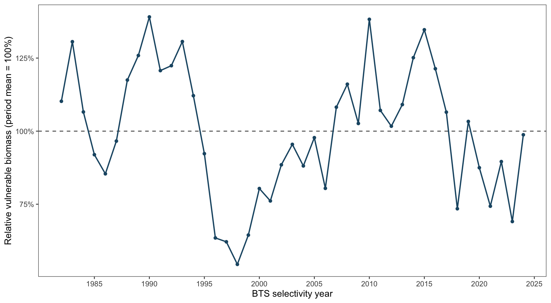
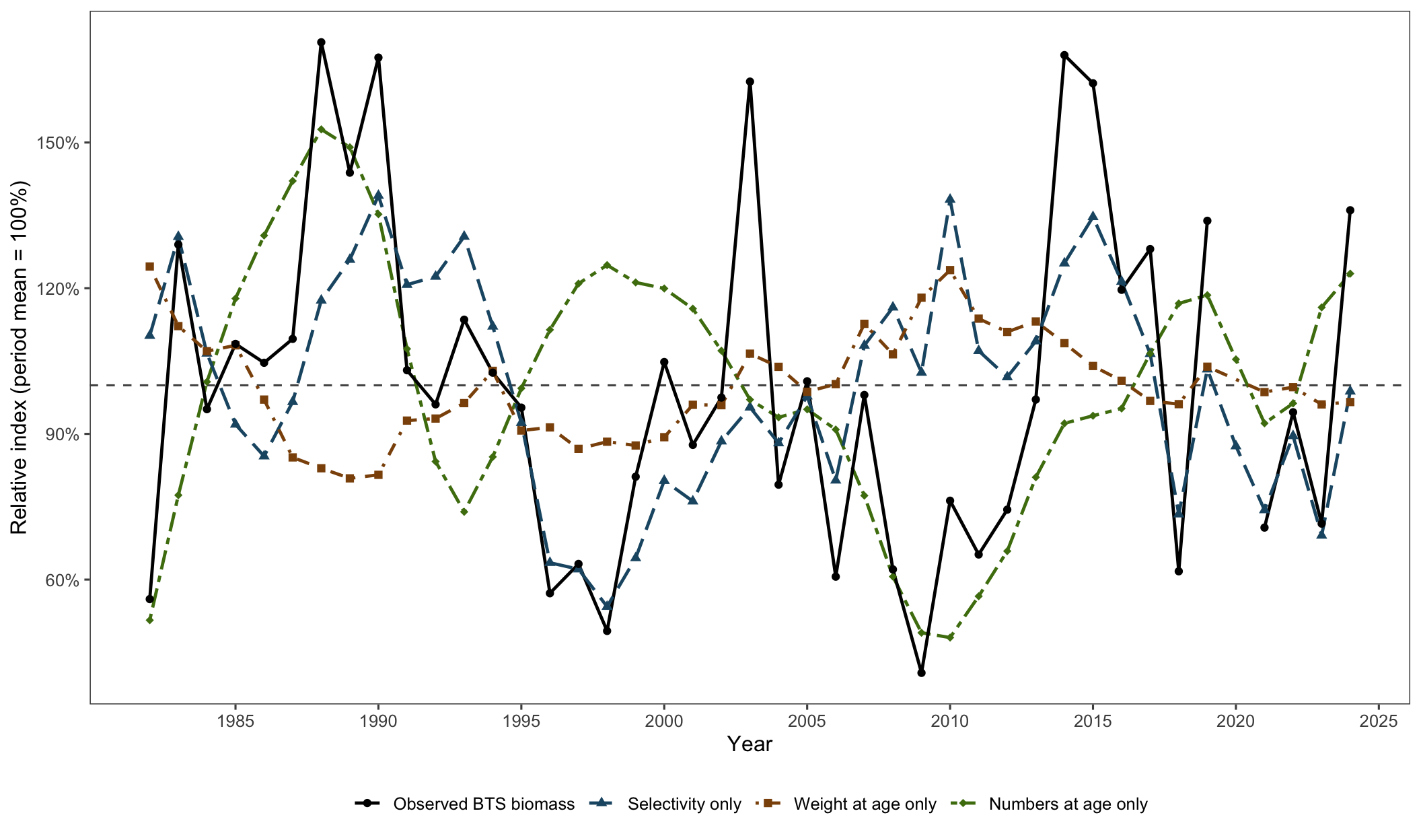
With numbers and weights fixed, the selectivity-only index in Figure 28 ranges from 54.4% to 139.1% of its period mean. Thus, fitted BTS selectivity alone produces deviations of approximately -45.6% to 39.1% around mean vulnerable biomass. This range describes changes in modeled survey availability caused by selectivity. Population biomass change is outside this controlled calculation.
An analogous weight-only calculation holds mean estimated numbers at age and BTS selectivity fixed. Selectivity is averaged at each age over 1982–2024, while the observed BTS weight-at-age vector varies among the 42 survey years. The 2020 survey was absent, so the plotted BTS weight series moves directly from 2019 to 2021.
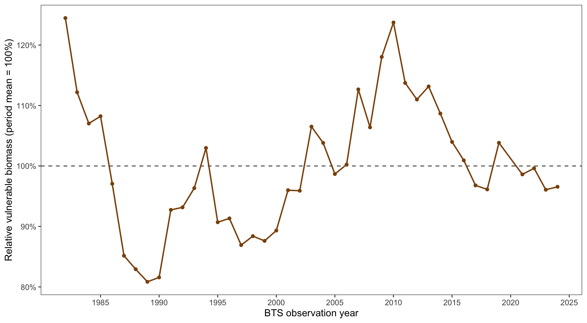
With mean estimated numbers at age and mean selectivity fixed, annual BTS weights alone produce the relative vulnerable-biomass range shown in Figure 29, from 80.8% to 124.5%, equivalent to deviations of -19.2% to 24.5% around the mean.
The third calculation holds both BTS selectivity and BTS weight at age at their period means and varies only the model-estimated numbers at ages 1–15. It therefore describes how the estimated population age structure and scale would change BTS-vulnerable biomass under a constant observation process.
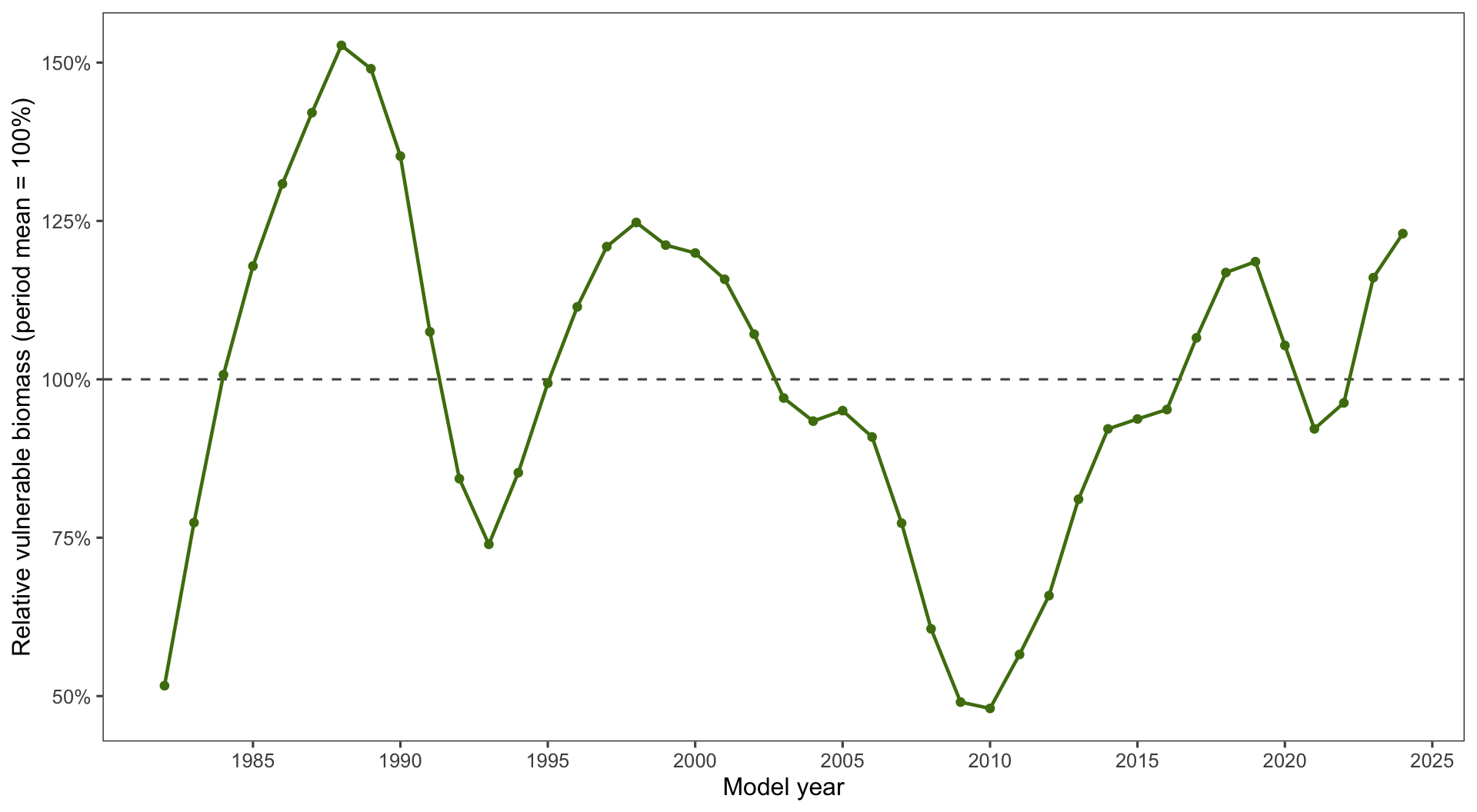
With mean selectivity and mean weight fixed, estimated numbers at age alone produce the relative vulnerable-biomass range shown in Figure 30, from 48.1% to 152.7%, equivalent to deviations of -51.9% to 52.7% around the mean. Unlike the first two controlled calculations, this third series reflects estimated population change rather than observation-process variation.
The combined comparison in Figure 31 places the three controlled series from Figure 28, Figure 29, and Figure 30 on the same scale as the observed BTS biomass index. Each series is divided by its own period mean, so 100% represents the mean for that series rather than a common biomass level. The BTS observation series retains the 2020 survey gap.
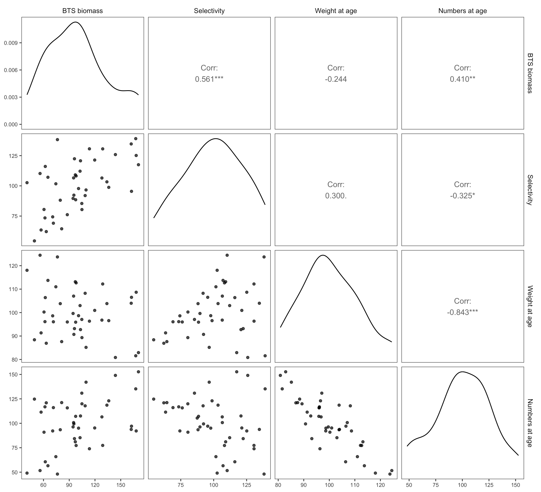
The pairwise display in Figure 32 removes the time axis and compares the four normalized series directly. Diagonal panels show each marginal distribution, lower panels show paired annual values, and upper panels report Pearson correlations based on the years available for each pair. These correlations describe shared temporal variation among the normalized indices. The controlled calculations leave causal contributions to observed survey biomass undetermined.
Appendix 4: Exploratory SparseNUTS sampling
This appendix evaluates whether the complete Model 26.0 joint objective can be sampled with SparseNUTS. It uses the same 1964–2024 input data and operating configuration as the maximum-likelihood fit: DSEM is set to NULL, recruitment deviations are represented as fixed parameters, and the full set of 1,218 joint parameters enters the sampler. The four dense-metric chains each used 1,000 warmup iterations followed by 1,000 retained draws, for 4,000 retained draws in total. The chains began at the converged maximum-likelihood estimates, where the maximum absolute gradient was 0.000050.
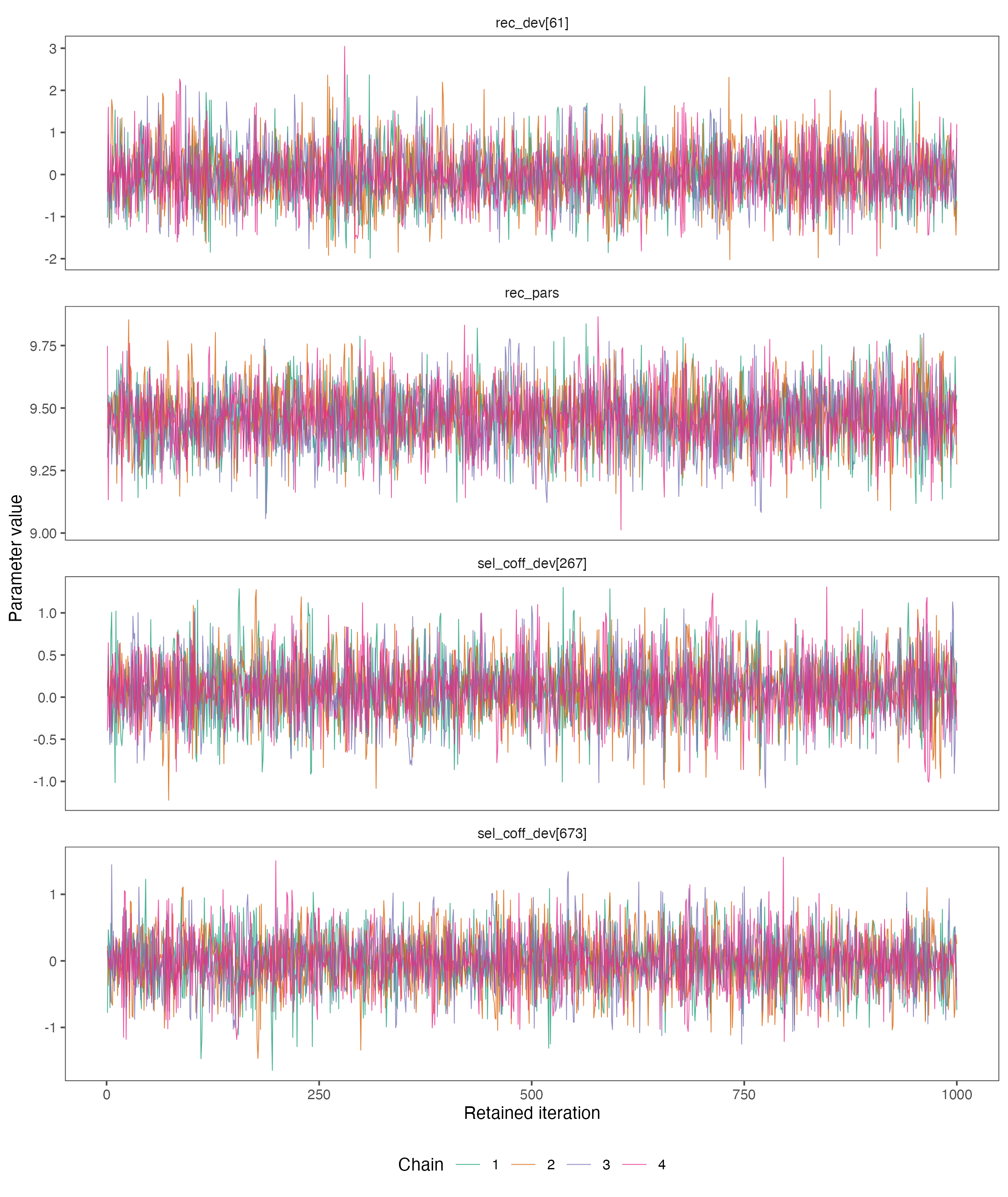
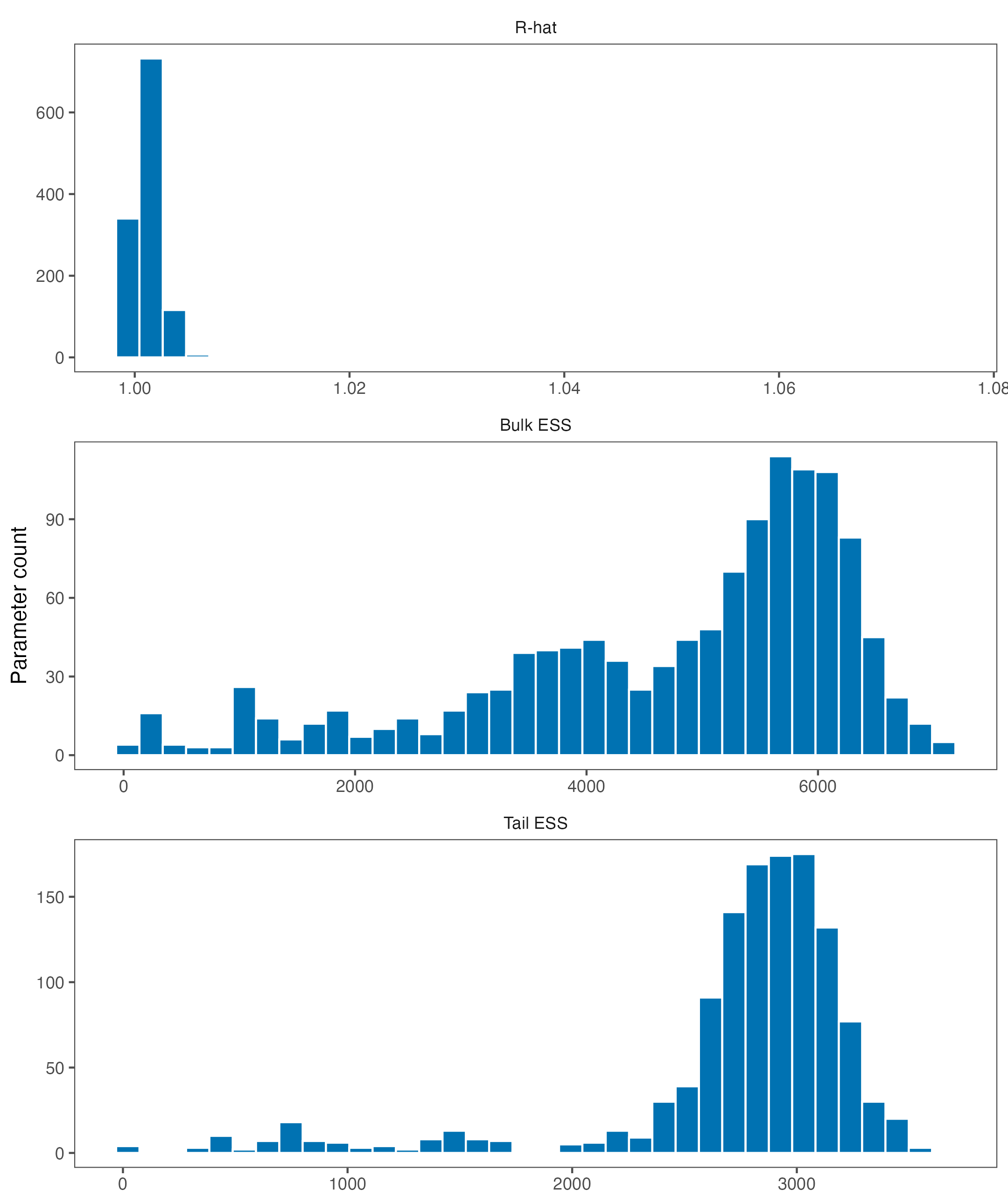
The run completed with zero divergences, zero maximum-tree-depth events, and a minimum energy Bayesian fraction of missing information (E-BFMI) of 1.001. Minimum tail effective sample size (ESS) was 22. Maximum R-hat was 1.075 and minimum bulk ESS was 36; both occurred for log_sel_slp_dev[7] and fall outside the review targets of R-hat at or below 1.01 and ESS at or above 400. The trace examples show representative parameters, while the full diagnostic distribution identifies incomplete mixing for a group of selectivity-change parameters (Figure 33; Figure 34; Table 19).
Energy Bayesian fraction of missing information (E-BFMI): measures how effectively momentum resampling moves a Hamiltonian Monte Carlo chain across the energy levels of its joint position-and-momentum distribution. It compares the squared change in total energy between successive iterations with the overall variation in energy. In plain language, E-BFMI asks whether each step changes energy enough to explore the posterior landscape. Higher values support more effective energy exploration. Values below 0.30 are commonly treated as a warning rather than a universal pass-or-fail threshold (Betancourt 2016, 2017). The CmdStan diagnostic guide uses 0.30 as its nominal warning threshold.
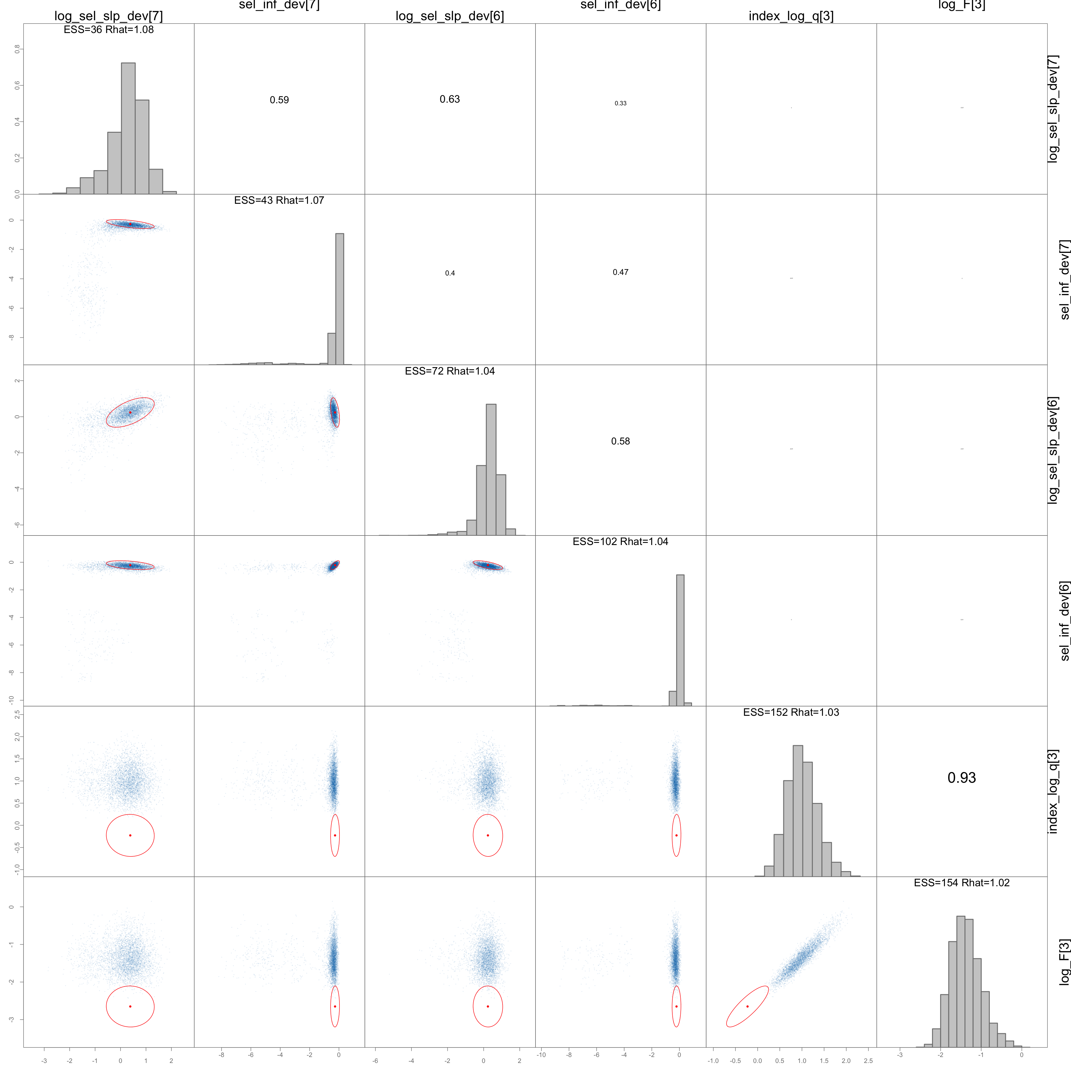
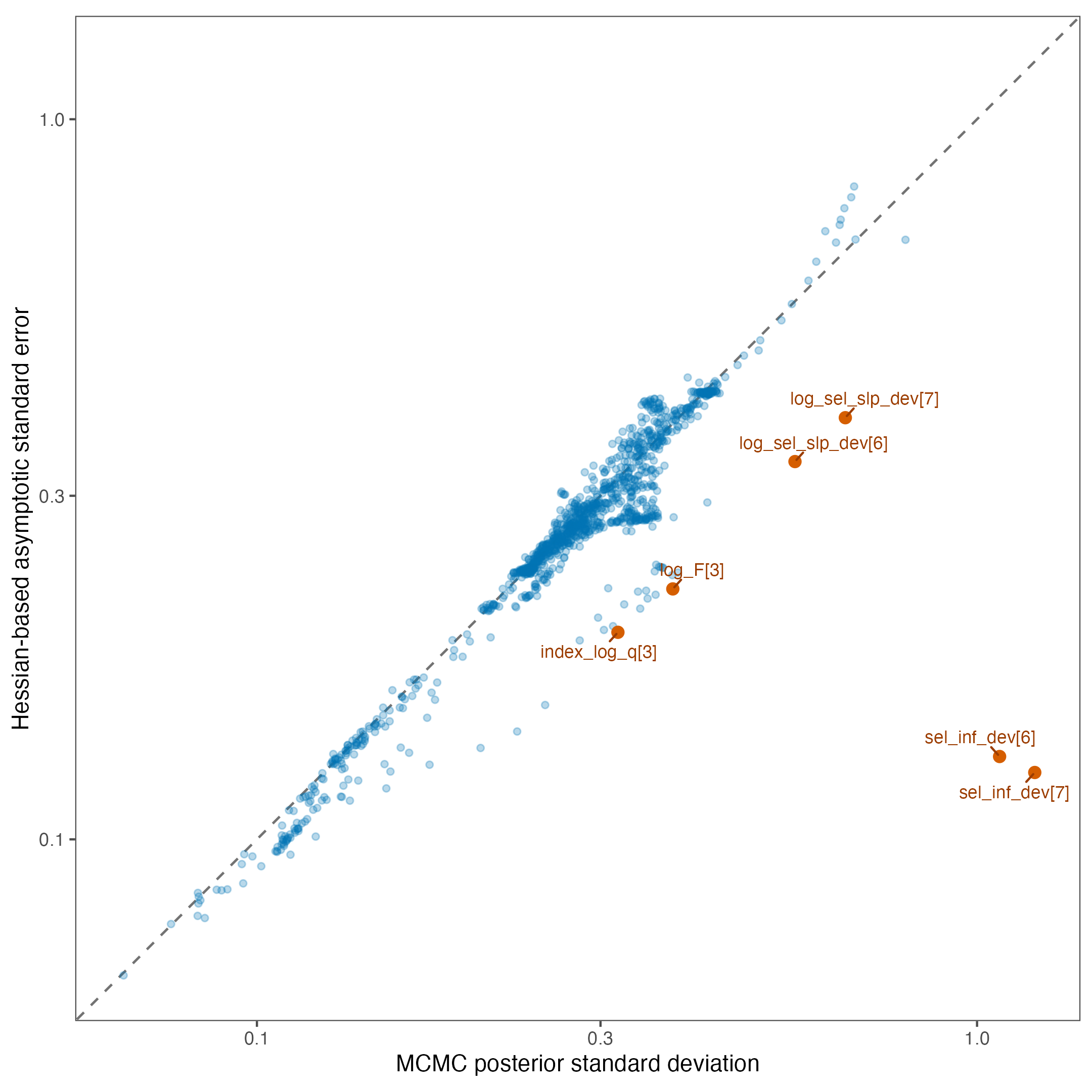
The six parameters with the lowest bulk ESS were log_sel_slp_dev[7], sel_inf_dev[7], log_sel_slp_dev[6], sel_inf_dev[6], index_log_q[3], and log_F[3]. Their marginal and joint posterior distributions, pairwise correlations, maximum-likelihood estimates, and Hessian-based correlation ellipses are shown in Figure 35. The uncertainty comparison in Figure 36 compares posterior standard deviations from the retained draws with local asymptotic standard errors derived from the maximum-likelihood Hessian for all 1,218 parameters. The dashed one-to-one line marks agreement between the two uncertainty summaries. The pairwise posterior correlations among the six slowest-mixing parameters range from -0.01 to 0.93. Across all parameters, the log-scale correlation between MCMC and Hessian uncertainty is 0.939, and the median ratio of MCMC standard deviation to Hessian standard error is 1.012. The corresponding ratios for the six slowest parameters range from 1.64 to 9.71. Differences from the one-to-one line can reflect posterior shape as well as sampling behavior, so this figure is interpreted together with R-hat, ESS, trace, and pairs diagnostics.
These results demonstrate the mechanics for sampling the complete joint objective on four local cores. The mixing diagnostics support reparameterizing the annual selectivity changes and testing a longer, tuned run before using posterior summaries for inference. The SparseNUTS results therefore remain an exploratory evaluation and are separate from the maximum-likelihood Model 26.0 results proposed for management advice. The complete 87-MB fit object is retained in the local analysis results directory, while this report carries only compact diagnostic tables and figures. Script M26-10 reproduces the run from the saved Model 26.0 fit.
| Diagnostic | Result | Review target | Outcome |
|---|---|---|---|
| Chains | 4 | 4 | Pass |
| Warmup iterations per chain | 1,000 | 1,000 | Pass |
| Retained draws per chain | 1,000 | 1,000 | Pass |
| Maximum R-hat | 1.075 | 1.01 or lower | Review |
| Minimum bulk ESS | 36 | 400 or higher | Review |
| Minimum tail ESS | 22 | 400 or higher | Review |
| Divergences | 0 | 0 | Pass |
| Maximum-tree-depth events | 0 | 0 | Pass |
| Minimum E-BFMI | 1.001 | above 0.30 | Pass |
Appendix 5: Reproducible model run methods
The model workflow keeps the editable report and analysis code under version control while storing large fit objects in the local analysis repository. The Rceattle library is pinned to version 5.23.0 from commit adf22f84b399e84e3b9a707e0b3bbb1624179a27 on the dsem-v5-integration branch. This preserves the exact model code used for the results. Each script checks the expected package version before fitting. The base assessment specification uses the established nonparametric selectivity, omits the two-dimensional age-by-year AR1 option, sets DSEM to NULL, and retains recruitment deviations as fixed parameters.
The following sequence reproduces the analysis. First, install the pinned Rceattle revision and afscOSA 0.0.1 in an isolated R library. Second, run M23-01 when the ADMB-to-Rceattle translation check needs rebuilding. Third, from the analysis repository, run M26-01; it reads the 1964–2024 assessment workbook, fits the model in two stages, saves the complete fit locally, and creates the bridge, OSA, and jitter products. Fourth, run M26-02 through M26-04 for the self-test and lag-preserving retrospective evaluations. Fifth, run M26-09 and M26-11 for whole-index and sampling-event influence. Sixth, run M26-05 followed by M26-06 for the spmR projection handoff. Finally, run the research evaluations M26-07 and M26-10 separately from the operational fit, then run M26-12 to summarize the retained SparseNUTS draws. Run M26-13 after M26-01 to rebuild the fitted index and age-composition displays from the saved Model 26.0 object.
The shell pattern below makes the analysis and report locations explicit. The scripts write complete fit objects beneath the analysis repository’s results/ directory and compact report products beneath the report source tree.
The script register in Table 20 gives the stable ID, purpose, input, and output for every step. These IDs provide a short reference for reruns, review notes, and archived products.
| Step | Script ID | Script | Purpose |
|---|---|---|---|
| 1 | M23-01 | run_model_23_0_vs_23_2_admb_comparison.R | Rebuild and compare the original and Rceattle-aligned ADMB bridge runs |
| 2 | M26-01 | run_model_26_rceattle_5_23.R | Fit the two-stage Model 26.0 base and create bridge OSA and jitter diagnostics |
| 3 | M26-02 | run_model_26_self_test_5_23.R | Simulate and refit the configured model for parameter and state recovery |
| 4 | M26-03 | run_model_26_retrospective_sensitivity_5_23.R | Run nine peels with stream-specific data lags and terminal selectivity treatment |
| 5 | M26-04 | run_model_26_retrospective_data_sensitivity_5_23.R | Test observation blocks responsible for the 2020–2021 retrospective transition |
| 6 | M26-09 | run_model_26_index_series_sensitivity_5_23.R | Refit after removing the complete BTS ATS or AVO fleet contribution while retaining CPUE |
| 7 | M26-05 | write_spmr_projection_inputs.R | Translate the fitted population state and biological schedules into SPM files |
| 8 | M26-06 | run_model_26_spmr_projection_5_23.R | Run and summarize the seven Tier 3 projection alternatives |
| 9 | M26-07 | run_model_26_dsem_5_23_pathways.R | Fit the separate exploratory recruitment-pathway models |
| 10 | M26-10 | run_model_26_sparsenuts_5_23.R | Sample the complete joint Model 26.0 objective with four dense-metric chains |
| 11 | M26-11 | run_model_26_case_deletion_5_23.R | Build the observation schedule and refit after deleting selected complete sampling events |
| 12 | M26-12 | plot_model_26_sparsenuts_diagnostics.R | Create pairs and uncertainty-comparison diagnostics from the retained SparseNUTS draws |
| 13 | M26-13 | plot_model_26_fits.R | Create fitted index and annual age-composition displays from the active Model 26.0 rows |
Appendix 6: Observation continuity and case-deletion influence
This diagnostic separates whether an observation was available and used from how much the accepted fit changes when a fitted sampling event is removed. The observation-continuity panel uses an explicit assessment-input schedule: annual for the fishery, BTS, and AVO rows and even years for ATS rows. Years after 2024 are shown only to distinguish the current fitted span; the schedule does not imply a commitment about future field operations.
The continuity panel distinguishes events present in the Model 26.0 input, scheduled events that are absent, years outside a row’s fitted span, and years after the terminal fitted year (Figure 37). It also shows where age-1 proportions are fitted separately from the main age composition. This makes survey timing, composition coverage, and recent gaps visible without treating the schedule as a prediction.
The case-deletion analysis removes an entire fitted index observation or composition row for one selected fleet-year event and then refits the complete model. All 11 refits reached convergence status OK with positive-definite Hessians. The 2024 BTS biomass index had the largest terminal spawning biomass effect (-5.28%) and lowered terminal age-1 recruitment by 25.31%. Removing the 2024 ATS age composition lowered terminal spawning biomass by 2.66% and raised terminal recruitment by 25.48%; its largest recruitment change across all years was 54.24%. Removing the 2024 AVO index raised terminal spawning biomass by 5.10% and terminal recruitment by 5.93%. Other selected events produced smaller terminal changes (Figure 38; Table 21).
These values describe influence within the current fitted model. Decisions about observation weighting draw on the full data-quality record, sampling design, fit diagnostics, and biological interpretation. Script M26-11 creates the explicit schedule, refits the selected cases, and saves each compact checkpoint locally.
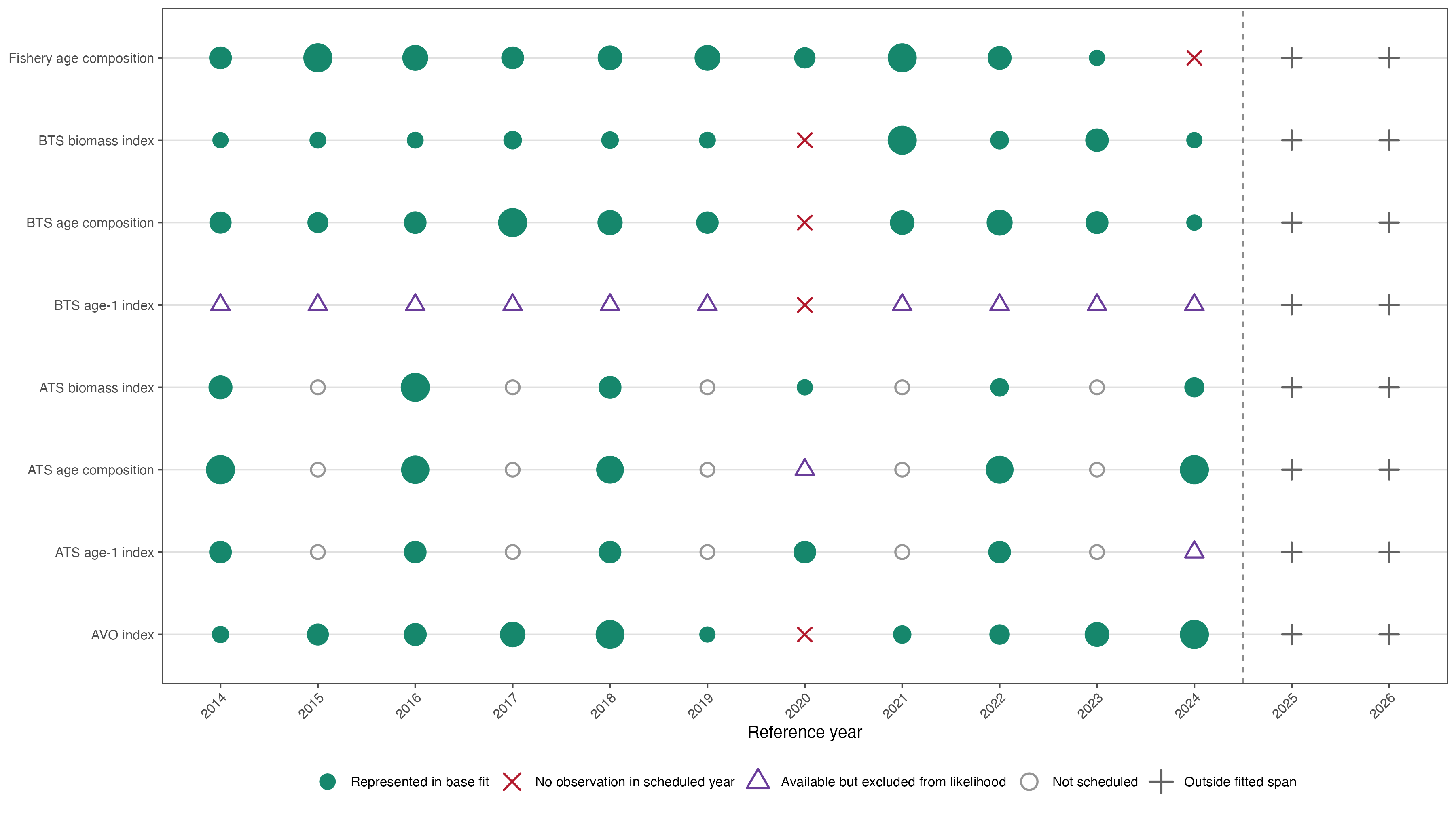
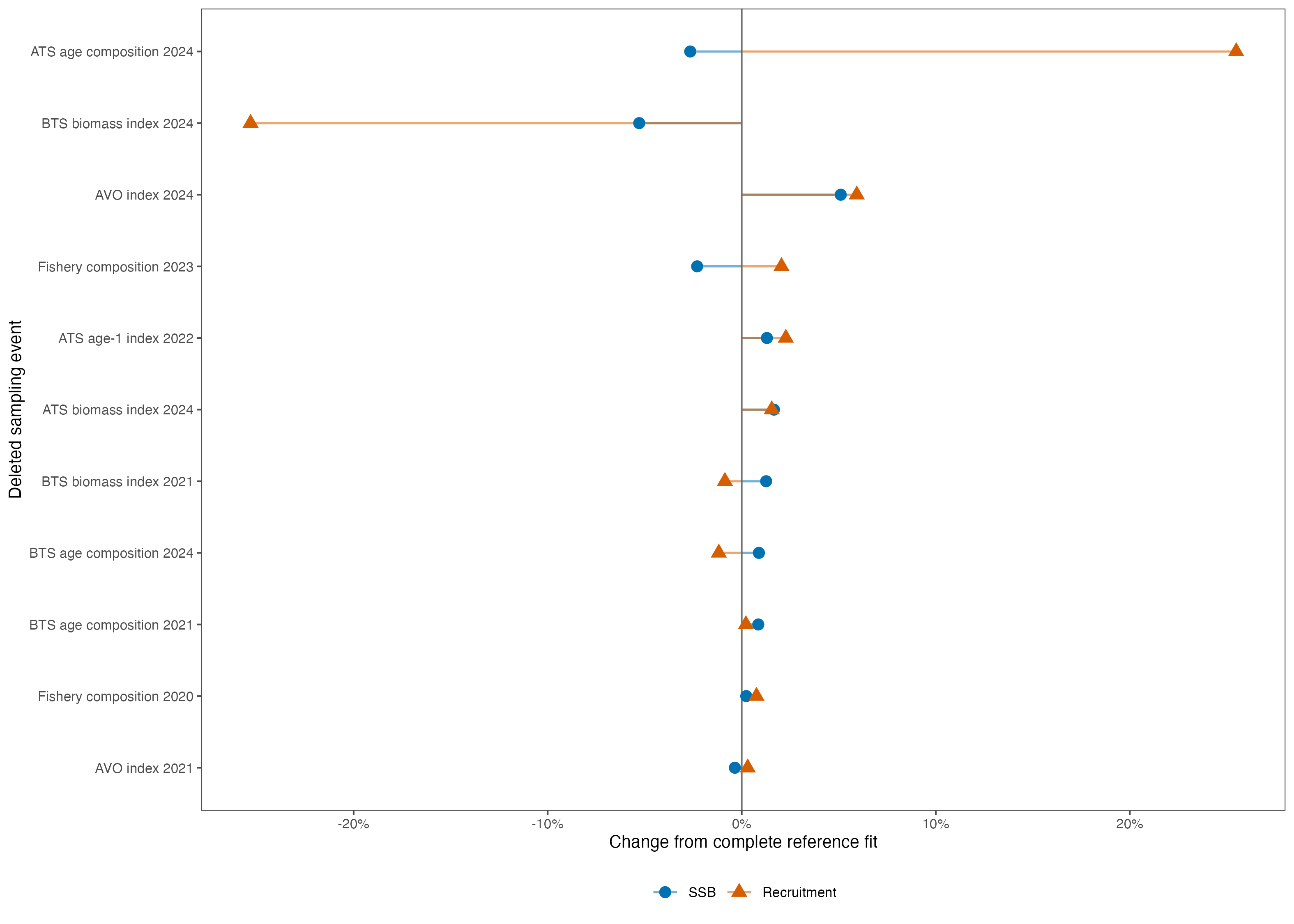
| Sampling event removed | Terminal SSB change (%) | Terminal recruitment change (%) | Largest recruitment change (%) |
|---|---|---|---|
| Fishery composition 2020 | +0.23 | +0.76 | 14.50 |
| Fishery composition 2023 | -2.30 | +2.05 | 11.71 |
| BTS biomass index 2021 | +1.26 | -0.87 | 1.39 |
| BTS biomass index 2024 | -5.28 | -25.31 | 25.31 |
| BTS age composition 2021 | +0.85 | +0.21 | 7.48 |
| BTS age composition 2024 | +0.88 | -1.18 | 15.77 |
| ATS biomass index 2024 | +1.66 | +1.55 | 2.47 |
| ATS age composition 2024 | -2.66 | +25.48 | 54.24 |
| ATS age-1 index 2022 | +1.30 | +2.27 | 8.65 |
| AVO index 2021 | -0.35 | +0.31 | 0.56 |
| AVO index 2024 | +5.10 | +5.93 | 9.90 |
Appendix 7: Glossary of acronyms
This glossary follows the ASAR package convention of maintaining one alphabetical source table with Label, Acronym, and Meaning fields. The label provides a stable key for document automation, while the acronym and meaning provide the reader-facing text. The report-specific source file can be updated once and reused in future output formats (Table 22).
| Acronym | Meaning | |
|---|---|---|
| 1 | ABC | acceptable biological catch |
| 2 | ADMB | Automatic Differentiation Model Builder |
| 3 | AFSC | Alaska Fisheries Science Center |
| 4 | AI | artificial intelligence |
| 5 | AIC | Akaike information criterion |
| 6 | AR1 | first-order autoregressive structure |
| 7 | ATS | acoustic-trawl survey |
| 8 | AVO | acoustic vessel-of-opportunity |
| 9 | B35% | spawning biomass reference point associated with 35 percent of unfished spawning potential |
| 10 | B40% | spawning biomass reference point associated with 40 percent of unfished spawning potential |
| 11 | BSAI | Bering Sea and Aleutian Islands |
| 12 | BTS | bottom-trawl survey |
| 13 | CEATTLE | Climate-enhanced Age-based model with Temperature-specific Trophic Linkages and Energetics |
| 14 | CPUE | catch per unit effort |
| 15 | DSEM | dynamic species environment model |
| 16 | E-BFMI | energy Bayesian fraction of missing information |
| 17 | EBS | eastern Bering Sea |
| 18 | ESP | Ecosystem and Socioeconomic Profile |
| 19 | ESR | Ecosystem Status Report |
| 20 | ESS | effective sample size |
| 21 | FT-NIR | Fourier-transform near-infrared method |
| 22 | FT-NIRS | Fourier-transform near-infrared spectroscopy |
| 23 | GOA | Gulf of Alaska |
| 24 | HMC | Hamiltonian Monte Carlo |
| 25 | ISS | input sample size |
| 26 | LR | likelihood ratio |
| 27 | MCMC | Markov chain Monte Carlo |
| 28 | MLE | maximum-likelihood estimate |
| 29 | NLL | negative log likelihood |
| 30 | NOAA | National Oceanic and Atmospheric Administration |
| 31 | NPFMC | North Pacific Fishery Management Council |
| 32 | NUTS | no-U-turn sampler |
| 33 | OFL | overfishing limit |
| 34 | OSA | one-step-ahead |
| 35 | Q-Q | quantile-quantile |
| 37 | R-hat | rank-normalized potential scale-reduction statistic |
| 36 | Rceattle | R implementation of CEATTLE |
| 38 | RTMB | R Template Model Builder |
| 39 | SAFE | Stock Assessment and Fishery Evaluation |
| 40 | SDNR | standard deviation of normalized residuals |
| 41 | SparseNUTS | sparse-matrix implementation of the no-U-turn sampler |
| 42 | SPM | Standard Projection Model |
| 43 | SPR | spawning potential ratio |
| 44 | SRR | stock-recruit relationship |
| 45 | SSB | spawning stock biomass |
| 46 | SSC | Scientific and Statistical Committee |
| 47 | SST | sea-surface temperature |
| 48 | TMB | Template Model Builder |
Appendix 8: Fishery length frequency patterns
This appendix summarizes exploratory seasonal and spatial patterns in observed pollock length-frequency samples. Its scope is exploratory description; assessment-model tests belong in separate analyses. The source analysis includes pollock observations from 1991 onward, excludes observations below 20 cm, and accumulates fish 65 cm and longer in a 65-cm-plus group. Length frequencies are normalized within each displayed year and grouping. A season includes samples collected before June 20; B season data are from June 20 onward. Earlier years appear at the top of each figure.
6.0.1 Change from 2025 to 2026
The observed length distribution shifted toward smaller fish from 2025 to 2026. Across seasons, mean sampled length declined from 46.17 to 44.81 cm, while the median remained 46 cm. The percentage longer than 46 cm decreased from 46.40% to 43.96%, and the percentage at or below 35 cm increased from 4.03% to 9.86%.
The shift occurred primarily in the B-season samples. B-season mean length declined from 45.93 cm in 2025 to 42.55 cm in 2026, and the median declined from 46 to 43 cm. The proportion longer than 46 cm decreased from 48.90% to 34.76%, while the proportion at or below 35 cm increased from 6.79% to 17.54%. Both B-season area groups shifted toward smaller fish. In the western group (NMFS_AREA > 519), mean length declined from 44.26 to 39.39 cm and the percentage at or below 35 cm increased from 9.86% to 29.24%. In the eastern group (NMFS_AREA < 520), mean length declined from 48.55 to 45.62 cm and the percentage longer than 46 cm decreased from 70.13% to 49.88%.
The A-season change was smaller and differed in shape. Mean length declined from 46.39 to 45.82 cm and the median remained 46 cm, while the percentages longer than 46 cm and at or below 35 cm both increased. This indicates greater representation in the tails of the sampled A-season distribution in 2026. Sample coverage also changed: the A-season count increased from 91,912 to 101,038 observations, whereas the B-season count decreased from 80,749 to 45,057. These are unstandardized sample distributions, so the differences describe the available observations and may reflect changes in sampling as well as changes in the fish encountered by the fishery.
6.0.2 A- and B-season distributions
The seasonal distributions show the larger 2026 shift toward smaller fish in the B season and the broader-tailed A-season pattern (Figure 39).
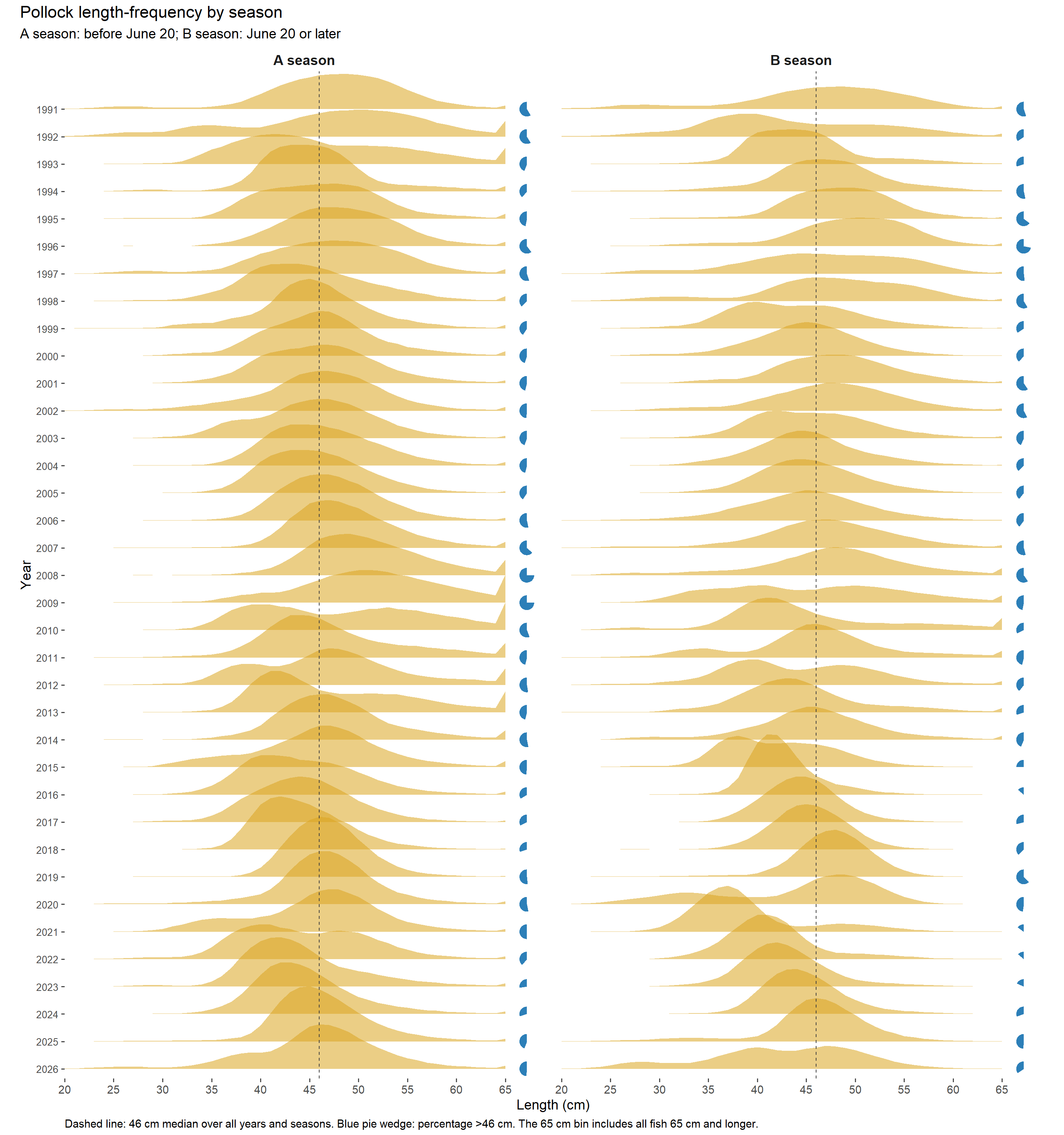
6.0.3 Combined-season distributions
The combined-season series places the 2026 increase in fish at or below 35 cm within the longer record of annual sample distributions (Figure 40).
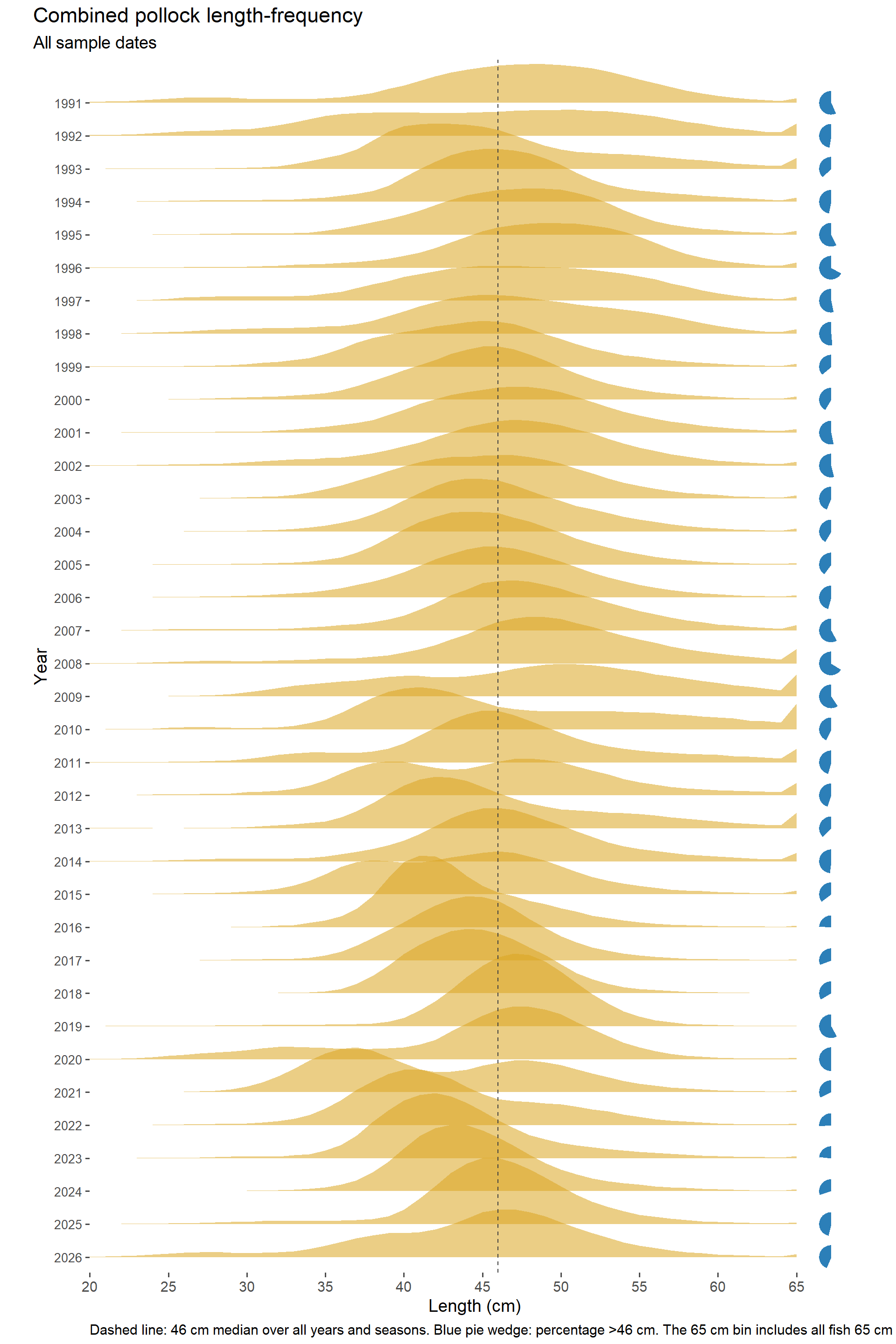
6.0.4 B-season distributions by NMFS area
The B-season area comparison shows a stronger shift toward smaller fish in the western group, while the eastern group retains a larger share above 46 cm (Figure 41).
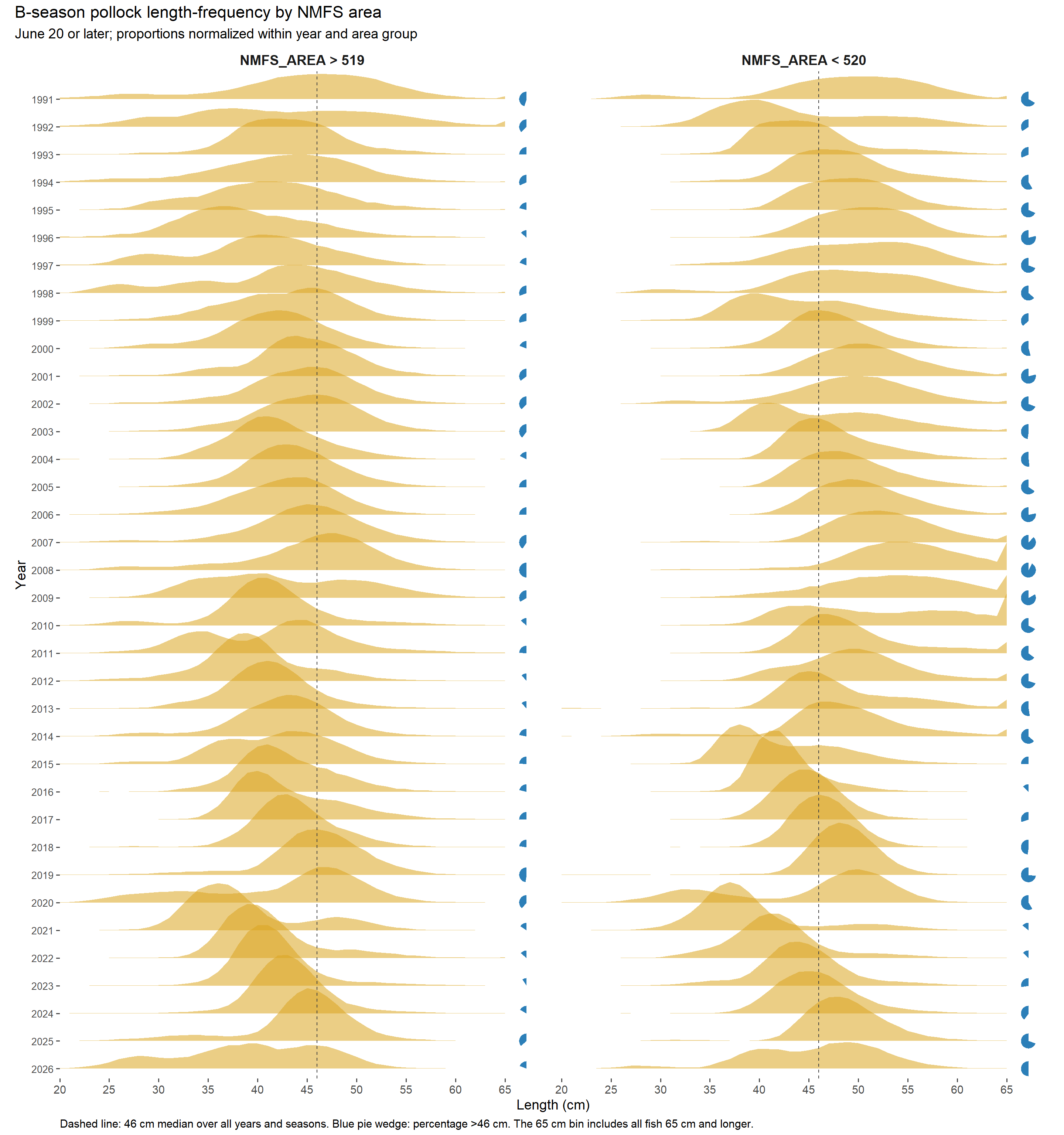
Comments and responses
The response matrix pairs each October 2025 SSC comment with the analysis, documentation, or review action planned for the 2026 assessment cycle.
sdmTMBbiomass estimates andtinyVASTage compositions as updated survey data. Record the data delivery date, software version, model settings, and input files. Compare the old and new survey series and show whether the change affects the assessment results.