Implementing parameter transformations in SNUTS

library(SparseNUTS)
library(RTMB)

One major difference with the Stan and ADMB platforms is that SNUTS does not natively handle parameter transformations such as box constraints. StanEstimator::stan_sample has arguments for lower and upper bounds of parameters, but this functionality is not compatible with SNUTS because the decorrelation happens prior to applying the transformations. Instead, the analyst must do this manually in the model code, and include a Jacobian manually as needed.

This article demonstrates how to implement parameter transformations in RTMB for strictly positive parameters (e.g., variances) as well as a box constraint with a lower and upper bound (e.g., a probability). These are based on the Jacobians defined here. A similar approach would be used in TMB as well.

When is a Jacobian necessary? According to the Stan manual: ‘A transformation samples a parameter, then transforms it, whereas a change of variables transforms a parameter, then samples it. Only the latter requires a Jacobian adjustment.’

The model below demonstrates how to use Jacobians and what happens if you do not include them. The overall idea is to define several parameters with different transformations (log and logit) and put explicit priors on them in a model without data. Then the posterior samples will be from the priors and an analytical posterior known. Specifically, each parameter is duplicated to include (right) or not (wrong) the Jacobian, and the model is then integrated to show the change in the posterior that results. Note that the Jacobians are added to the log-density and negated at the end. A user can copy the Jacobians used here to account for this change-of-variable scenario. Just be mindful of getting the sign right!

library(SparseNUTS)
library(RTMB)
# parameters in the transformed space
pars <- list(log_sigma_right=0, log_sigma_wrong=0,
             logit_p_right=0, logit_p_wrong=0,
             logit_box_right=0, logit_box_wrong=0)
dat <- list(mu1=10, sd1=2,
            shape1=2, shape2=8,
            a=0, b=8,
            s2=2, r2=2)
            #mu2=50, sd2=20)
func <- function(pars){
  getAll(pars, dat)
  # transform the parameters
  sigma_right <- exp(log_sigma_right)
  sigma_wrong <- exp(log_sigma_wrong)
  # these are constrained to be in (0,1)
  p_right <- plogis(logit_p_right)
  p_wrong <- plogis(logit_p_wrong)
  # constrained in (a,b)
  box_right <- a + (b-a)*plogis(logit_box_right)
  box_wrong <- a + (b-a)*plogis(logit_box_wrong)
  # add priors *after* inverse transformation
  lp <- dnorm(sigma_right, mean=mu1, sd=sd1, log=TRUE) +
    dnorm(sigma_wrong, mean=mu1, sd=sd1, log=TRUE) +
    dbeta(p_right, shape1=shape1, shape2=shape2, log=TRUE)+
    dbeta(p_wrong, shape1=shape1, shape2=shape2, log=TRUE)+
    # this is a truncated gamma since bounded (a,b)
    dgamma(box_right, shape=s2, rate=r2, log=TRUE) +
    dgamma(box_wrong, shape=s2, rate=r2, log=TRUE)
 # add Jacobians to the "right" ones
  tmp <- plogis(logit_box_right)
  lp <- lp + log_sigma_right +
    log(p_right*(1-p_right)) +
    log((b-a)*tmp*(1-tmp))
  # note the lack of jacobians for the "wrong" ones
  REPORT(sigma_right); REPORT(sigma_wrong)
  REPORT(p_right); REPORT(p_wrong)
  REPORT(box_right); REPORT(box_wrong)
  return(-lp)
}
func(pars)
#> [1] 37.15916
obj <- MakeADFun(func, parameters=pars)

Posterior samples can then be drawn using SNUTS.

fit <- sample_snuts(obj, seed=1, chains=1, refresh=0,
                    num_samples=5000, model_name='jacobian_test')
#> Optimizing...
#> Rebuilding RTMB obj without random effects...
#> diag metric selected b/c low correlations (max=0)
#> log-posterior at inits=(-1.42); at conditional mode=-1.416
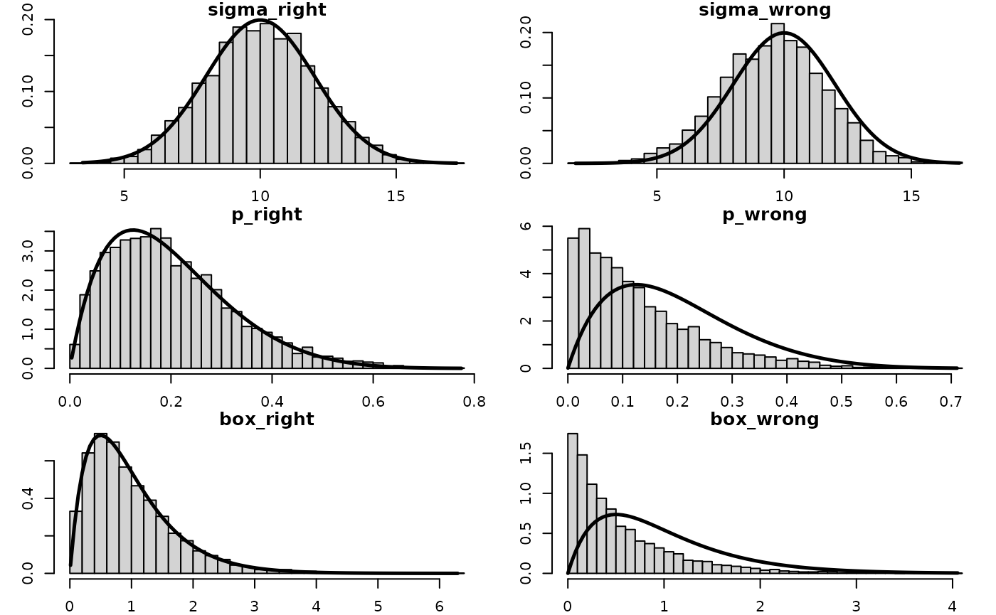
#> Starting MCMC sampling...

And then the posterior compared to the known truth (the priors), with and without the Jacobian adjustments. Without the Jacobian the posterior is wrong because the change in volume from the transformation is not accounted for.

post <- as.data.frame(fit)
xx <- apply(post, 1, \(i) obj$report(as.numeric(i)) |> unlist()) |> t() |>
  as.data.frame()
par(mfrow=c(3,2), mar=c(2,3,1,1))
lwd <- 2.5
breaks <- 40
hist(xx$sigma_right, xlab='', main='sigma_right', breaks=breaks,
     freq=FALSE)
curve(dnorm(x, mean=dat$mu1, sd=dat$sd1),
      from=min(xx$sigma_right),
      to=max(xx$sigma_right), add=TRUE, lwd=lwd)
hist(xx$sigma_wrong, xlab='n', main='sigma_wrong',breaks=breaks,
     freq=FALSE)
curve(dnorm(x, mean=dat$mu1, sd=dat$sd1),
      from=min(xx$sigma_wrong),
      to=max(xx$sigma_wrong), add=TRUE, lwd=lwd)

hist(xx$p_right, xlab='', main='p_right', breaks=breaks,
     freq=FALSE)
curve(dbeta(x, shape1=dat$shape1, shape2=dat$shape2),
      from=min(xx$p_right),
      to=max(xx$p_right), add=TRUE, lwd=lwd)
hist(xx$p_wrong, xlab='', main='p_wrong',breaks=breaks,
     freq=FALSE)
curve(dbeta(x, shape1=dat$shape1, shape2=dat$shape2),
      from=min(xx$p_wrong),
      to=max(xx$p_wrong), add=TRUE, lwd=lwd)
hist(xx$box_right, xlab='', main='box_right', breaks=breaks,
     freq=FALSE)
# technically a truncated gamma but tiny amount of mass outside
# bounds so ignoring it for plotting
curve(dgamma(x, shape=dat$s2, rate=dat$r2),
      from=min(xx$box_right),
      to=max(xx$box_right), add=TRUE, lwd=lwd)
hist(xx$box_wrong, xlab='', main='box_wrong', breaks=breaks,
     freq=FALSE)
curve(dgamma(x, shape=dat$s2, rate=dat$r2),
      from=min(xx$box_wrong),
      to=max(xx$box_wrong), add=TRUE, lwd=lwd)

Cole C. Monnahan

2026-02-11