The goal of SparseNUTS is to provide a user-friendly workflow for users of TMB and RTMB who want to implement the sparse no-u-turn sampler (Cole C. Monnahan et al. 2026) to draw samples from a model.
This package was originally developed inside of the adnuts package
but was split off in late 2025 to have a dedicated package for
SparseNUTS for TMB and RTMB models. The tmbstan package
(C. C. Monnahan and Kristensen 2018) also
provides an interface to the Stan software, but lacks the ability to
decorrelate the target distribution prior to sampling.
SparseNUTS provides more flexible options related to the
mass matrix.
Differences in usage between TMB and RTMB
Both TMB and RTMB models can be used with minimal user intervention,
including running parallel chains. The sample_snuts
function will detect which package is used internally and adjust
accordingly. If the user wants to use models from both packages in the
same session then one needs to be unloaded, e.g.,
if('TMB' %in% .packages()) detach(package:TMB), before the
other package is loaded.
If the RTMB model uses external functions or data sets then they must
be passed through via a list in the globals argument so
they are available to rebuild the ‘obj’ in the parallel R sessions.
Optionally, the model_name can be specified in the call,
otherwise your model will be labeled “RTMB” in the output. TMB models do
not require a globals input and the model name is pulled
from the DLL name, but can be overridden if desired.
Comparison to tmbstan
The related package ‘tmbstan’ (C. C. Monnahan
and Kristensen 2018) also allows users to link TMB models to the
Stan algorithms. ‘tmbstan’ links through the package ‘rstan’, while
‘SparseNUTS’ modifies the objective and gradient functions and then
passes those to ‘cmdstan’ through the ‘StanEstimators’ R package
interface. For models without large correlations or scale differences,
tmbstan is likely to be faster than ‘SparseNUTS’ due to
lower overhead and may be a better option. Eventually, Stan may add
SNUTS functionality and an interface to ‘tmbstan’ developed, and in that
case tmbstan may be a better long term option. For TMB
users now, SNUTS via SparseNUTS is likely to be the best
overall package for Bayesian inference.
SNUTS for TMB models from existing packages (sdmTMB, glmmTMB, etc.)
SparseNUTS works for custom TMB and RTMB models
developed locally, but also for those that come in packages. Most
packages will return the TMB ‘obj’ which can then be passed into
sample_snuts.
For instance the glmmTMB package can be run like
this:
library(glmmTMB)
library(SparseNUTS)
data(Salamanders)
obj <- glmmTMB(count~spp * mined + (1|site), Salamanders, family="nbinom2")$obj
fit <- sample_snuts(obj)
Basic usage
The recommended usage for TMB users is to let the
sample_snuts function automatically detect the metric to
use and the length of warmup period, especially for pilot runs during
model development.
I demonstrate basic usage using a very simple RTMB version of the eight schools model that has been examined extensively in the Bayesian literature. The first step is to build the TMB object ‘obj’ that incorporates priors and Jacobians for parameter transformations. Note that the R function returns the negative un-normalized log-posterior density.
library(RTMB)
library(SparseNUTS)
dat <- list(y=c(28,  8, -3,  7, -1,  1, 18, 12),
            sigma=c(15, 10, 16, 11,  9, 11, 10, 18))
pars <- list(mu=0, logtau=0, eta=rep(1,8))
f <- function(pars){
  getAll(dat, pars)
  theta <- mu + exp(logtau) * eta;
  lp <- sum(dnorm(eta, 0,1, log=TRUE))+ # prior
    sum(dnorm(y,theta,sigma,log=TRUE))+ #likelihood
    logtau                          # jacobian
  REPORT(theta)
  return(-lp)
}
obj <- MakeADFun(func=f, parameters=pars,
                 random="eta", silent=TRUE)
Posterior sampling with SNUTS
The most common task is to draw samples from the posterior density
defined by this model. This is done with the sample_snuts
function as follows:
fit <- sample_snuts(obj, refresh=0, seed=1,
                    model_name = 'schools',
                    cores=1, chains=1,
                    globals=list(dat=dat))
## Optimizing marginal posterior with 2 fixed effects and 8 random effects...## Getting Q and its stats...## Q is 62.22% sparse | Ratio of marginal SDs=6.5 | Max abs cor >=0.2927## Rebuilding RTMB obj without random effects...## dense metric selected b/c faster than sparse and high correlation (max=0.2927)## log-posterior at inits=(-36.13); at conditional mode=-34.661## Starting MCMC sampling...##
##
## Gradient evaluation took 8.3e-05 seconds
## 1000 transitions using 10 leapfrog steps per transition would take 0.83 seconds.
## Adjust your expectations accordingly!
##
##
##
## Elapsed Time: 0.088 seconds (Warm-up)
## 0.552 seconds (Sampling)
## 0.64 seconds (Total)
##
##
##
## Model 'schools' has 10 pars and was fit using SNUTS with a 'dense' metric
## 1 chain(s) of 1150 total iterations (150 warmup) were used
## Run time per chain: average= 0.64 and max= 0.64 seconds
## Min bulk ESS=125.3 (12.53%) [logtau] and maximum Rhat=1.011 [eta[3]]
## !! Warning: Signs of non-convergence found. Do not use for inference !!
## There were 0 divergences after warmupThe returned object fit (an object of ‘adfit’ S3 class)
contains the posterior samples and other relevant information for a
Bayesian analysis.
Here a ‘diag’ (diagonal) metric is selected and a very short warmup period of 150 iterations is used, with mass matrix adaptation in Stan disabled. See below for more details on mass matrix adaptation within Stan.
Notice that no optimization was done before calling
sample_snuts. When the model has already been optimized,
you can skip that by setting skip_optimization=TRUE, and
even pass in
and
via arguments Q and Qinv to bypass this step
and save some run time. This may also be required if the model
optimization routine internal to sample_snuts is
insufficient. In that case, the user should optimize prior to SNUTS
sampling. The returned fitted object contains a slot called
mle (for maximum likelihood estimates) which has the
conditional mode (‘est’), the marginal standard errors ‘se’, a joint
correlation matrix (‘cor’), and the sparse precision matrix
.
str(fit$mle)## List of 6
## $ nopar: int 10
## $ est : Named num [1:10] 7.92441 1.8414 0.47811 0.00341 -0.2329 ...
## ..- attr(*, "names")= chr [1:10] "mu" "logtau" "eta[1]" "eta[2]" ...
## $ se : Named num [1:10] 4.725 0.732 0.959 0.872 0.945 ...
## ..- attr(*, "names")= chr [1:10] "mu" "logtau" "eta[1]" "eta[2]" ...
## $ Q :Formal class 'dsCMatrix' [package "Matrix"] with 7 slots
## .. ..@ i : int [1:27] 0 1 2 3 4 5 6 7 8 9 ...
## .. ..@ p : int [1:11] 0 10 19 20 21 22 23 24 25 26 ...
## .. ..@ Dim : int [1:2] 10 10
## .. ..@ Dimnames:List of 2
## .. .. ..$ : chr [1:10] "mu" "logtau" "eta[1]" "eta[2]" ...
## .. .. ..$ : chr [1:10] "mu" "logtau" "eta[1]" "eta[2]" ...
## .. ..@ x : num [1:27] 0.0603 -0.0144 0.028 0.0631 0.0246 ...
## .. ..@ uplo : chr "L"
## .. ..@ factors :List of 2
## .. .. ..$ sPDCholesky:Formal class 'dCHMsimpl' [package "Matrix"] with 11 slots
## .. .. .. .. ..@ x : num [1:28] 1.1227 0.0173 -0.0552 1.3976 0.0451 ...
## .. .. .. .. ..@ p : int [1:11] 0 3 6 9 12 15 18 22 25 27 ...
## .. .. .. .. ..@ i : int [1:28] 0 6 9 1 6 9 2 6 9 3 ...
## .. .. .. .. ..@ nz : int [1:10] 3 3 3 3 3 3 4 3 2 1
## .. .. .. .. ..@ nxt : int [1:12] 1 2 3 4 5 6 7 8 9 10 ...
## .. .. .. .. ..@ prv : int [1:12] 11 0 1 2 3 4 5 6 7 8 ...
## .. .. .. .. ..@ type : int [1:6] 2 0 0 1 0 0
## .. .. .. .. ..@ colcount: int [1:10] 3 3 3 3 3 3 4 3 2 1
## .. .. .. .. ..@ perm : int [1:10] 9 8 7 6 5 4 0 2 3 1
## .. .. .. .. ..@ Dim : int [1:2] 10 10
## .. .. .. .. ..@ Dimnames:List of 2
## .. .. .. .. .. ..$ : chr [1:10] "mu" "logtau" "eta[1]" "eta[2]" ...
## .. .. .. .. .. ..$ : chr [1:10] "mu" "logtau" "eta[1]" "eta[2]" ...
## .. .. ..$ SPdCholesky:Formal class 'dCHMsuper' [package "Matrix"] with 10 slots
## .. .. .. .. ..@ x : num [1:100] 1.06 0 0 0 0 ...
## .. .. .. .. ..@ super : int [1:2] 0 10
## .. .. .. .. ..@ pi : int [1:2] 0 10
## .. .. .. .. ..@ px : int [1:2] 0 100
## .. .. .. .. ..@ s : int [1:10] 0 1 2 3 4 5 6 7 8 9
## .. .. .. .. ..@ type : int [1:6] 2 1 1 1 1 1
## .. .. .. .. ..@ colcount: int [1:10] 3 3 3 3 3 3 4 3 2 1
## .. .. .. .. ..@ perm : int [1:10] 9 8 7 6 5 4 0 2 3 1
## .. .. .. .. ..@ Dim : int [1:2] 10 10
## .. .. .. .. ..@ Dimnames:List of 2
## .. .. .. .. .. ..$ : chr [1:10] "mu" "logtau" "eta[1]" "eta[2]" ...
## .. .. .. .. .. ..$ : chr [1:10] "mu" "logtau" "eta[1]" "eta[2]" ...
## $ Qinv : NULL
## $ cor : num [1:10, 1:10] 1 0.0558 -0.1031 -0.2443 -0.114 ...
## ..- attr(*, "dimnames")=List of 2
## .. ..$ : chr [1:10] "mu" "logtau" "eta[1]" "eta[2]" ...
## .. ..$ : chr [1:10] "mu" "logtau" "eta[1]" "eta[2]" ...Diagnostics
The common MCMC diagnostics potential scale reduction (Rhat) and
minimum ESS, as well as the NUTS divergences (see diagnostics
section of the rstan manual), are printed to console by default or
can be accessed in more depth via the monitor slot:
print(fit)## Model 'schools' has 10 pars and was fit using SNUTS with a 'dense' metric
## 1 chain(s) of 1150 total iterations (150 warmup) were used
## Run time per chain: average= 0.64 and max= 0.64 seconds
## Min bulk ESS=125.3 (12.53%) [logtau] and maximum Rhat=1.011 [eta[3]]
## !! Warning: Signs of non-convergence found. Do not use for inference !!
## There were 0 divergences after warmup
fit$monitor |> str()## drws_smm [11 × 10] (S3: draws_summary/tbl_df/tbl/data.frame)
## $ variable: chr [1:11] "mu" "logtau" "eta[1]" "eta[2]" ...
## $ mean : num [1:11] 8.5371 1.4046 0.3463 -0.0702 -0.2308 ...
## $ median : num [1:11] 8.4999 1.611 0.3322 -0.0822 -0.2602 ...
## $ sd : num [1:11] 4.831 1.228 0.943 0.864 0.927 ...
## $ mad : num [1:11] 4.459 1.049 0.927 0.868 0.943 ...
## $ q5 : num [1:11] 0.56 -0.966 -1.199 -1.514 -1.712 ...
## $ q95 : num [1:11] 16.48 3.1 1.95 1.33 1.42 ...
## $ rhat : num [1:11] 1.001 0.999 1.004 1.001 1.011 ...
## $ ess_bulk: num [1:11] 265 125 1409 1144 604 ...
## $ ess_tail: num [1:11] 597.6 28.9 704.8 522.1 666.6 ...
## - attr(*, "num_args")= list()A specialized pairs plotting function is available
(formally called pairs_admb) to examine pair-wise behavior
of the posteriors. This can be useful to help diagnose particularly slow
mixing parameters. This function also displays the conditional mode
(point) and 95% bivariate confidence region (ellipses) as calculated
from the approximate covariance matrix
.
The parameters to show can be specified either vie a character vector
like pars=c('mu', 'logtau', 'eta[1]') or an integer vector
like pars=1:3, and when using the latter the parameters can
be ordered by slowest mixing (‘slow’), fastest mixing (‘fast’) or by the
largest discrepancies in the approximate marginal variance from
and the posterior samples (‘mismatch’). NUTS divergences are shown as
green points. See help and further information at
?pairs.adfit.
pairs(fit, order='slow')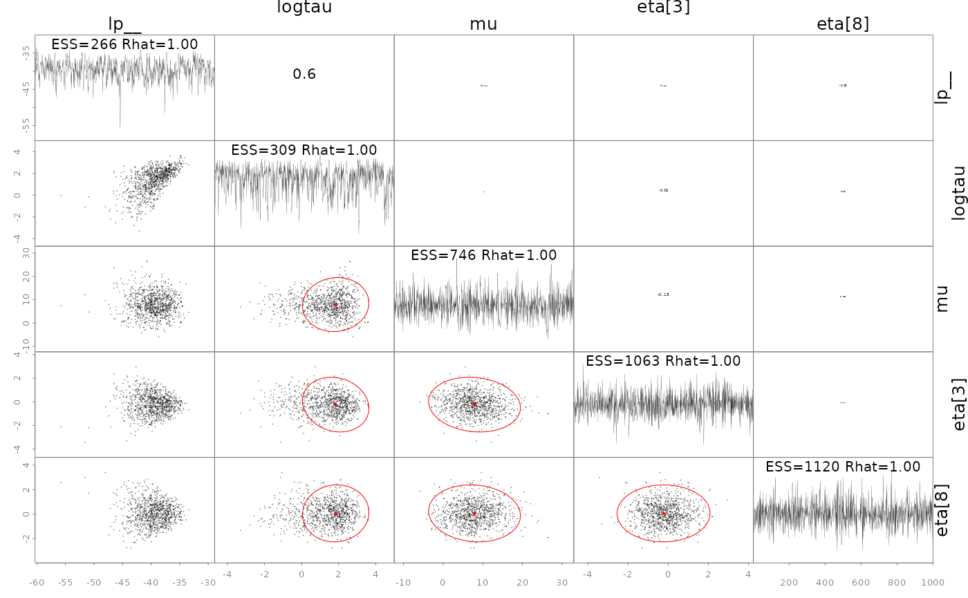
In some cases it is useful to diagnose the NUTS behavior by examining the “sampler parameters”, which contain information about the individual NUTS trajectories.
extract_sampler_params(fit) |> str()## 'data.frame': 1000 obs. of 8 variables:
## $ chain : num 1 1 1 1 1 1 1 1 1 1 ...
## $ iteration : num 151 152 153 154 155 156 157 158 159 160 ...
## $ accept_stat__: num 0.8 0.96 0.946 0.813 0.952 ...
## $ stepsize__ : num 0.502 0.502 0.502 0.502 0.502 ...
## $ treedepth__ : num 3 3 3 3 3 2 3 3 3 3 ...
## $ n_leapfrog__ : num 7 15 7 15 7 7 7 7 7 7 ...
## $ divergent__ : num 0 0 0 0 0 0 0 0 0 0 ...
## $ energy__ : num 42.9 45.8 46.5 49.8 48.5 ...
## or plot them directly
plot_sampler_params(fit)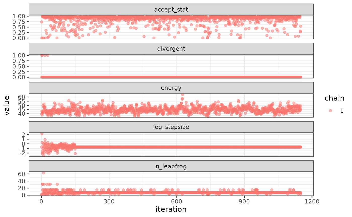
The ShinyStan tool is also available and provides a convenient,
interactive way to check diagnostics via the function
launch_shinytmb(), but also explore estimates and other
important quantities. This is a valuable tool for a workflow with
‘SparseNUTS’.
Bayesian inference
After checking for signs of non-convergence the results can be used
for inference. Posterior samples for parameters can be extracted and
examined in R by casting the fitted object to an R data.frame. These
posterior samples can then be put back into the TMB object
obj$report() function to extract any desired “generated
quantity” in Stan terminology. Below is a demonstration of how to do
this for the quantity theta (a vector of length 8).
post <- as.data.frame(fit)
post |> str()
## 'data.frame': 1000 obs. of 10 variables:
## $ mu : num 9.87 8.56 9.29 9.57 6.22 ...
## $ logtau: num 1.02 -1.99 -1.85 -1.54 -2.38 ...
## $ eta[1]: num 0.522 0.333 -0.252 -0.474 -0.967 ...
## $ eta[2]: num 0.986 -0.914 0.549 -0.332 -1.27 ...
## $ eta[3]: num -0.4304 0.0589 -0.0845 -0.4217 -0.591 ...
## $ eta[4]: num 1.741 0.962 -1.633 -1.333 -1.991 ...
## $ eta[5]: num -0.1247 -0.7945 0.1335 0.0112 0.5583 ...
## $ eta[6]: num -0.615 0.985 -2.11 -1.649 -0.3 ...
## $ eta[7]: num 0.404 1.194 -1.133 -2.022 -0.834 ...
## $ eta[8]: num 0.552 -1.207 0.906 0.957 0.654 ...
## now get a generated quantity, here theta which is a vector of
## length 8 so becomes a matrix of posterior samples
theta <- apply(post,1, \(x) obj$report(x)$theta) |> t()
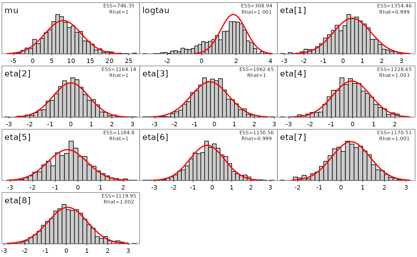
theta |> str()## num [1:1000, 1:8] 11.32 8.6 9.25 9.47 6.13 ...Likewise, marginal distributions can be explored visually and compared to the approximate estimate from the conditional mode and (red lines):
plot_marginals(fit)